[TOC]
参考
- 《Topological Insulators and Topological Superconductors》 - B. Andrei Bernevig
- Chapter-9 Time-Reversal-Invariant Topological Insulators
Chapter-9 Time-Reversal-Invariant Topological Insulators
The Haldane model of a Chern insulator shows that a nontrivial insulator with nonzero Hall conductance can exist when TR symmetry is broken. More than 15 years after the Haldane model was published, it was realized that keeping symmetries intact gives rise to systems as interesting as the ones where symmetries are broken. Kane and Mele \([4,5]\) first realized that by doubling the Haldane model of the Chern insulator by introducing spin in the problem, we can obtain an insulator that maintains TR symmetry but has a robust, gapless pair of helical (not chiral) edge states. In this chapter we introduce the Kane and Mele model first and then introduce the HgTe model [7] for a topological insulator. Such an insulator was the first experimentally realizable topological insulator, and its experimental discovery blew the field of topological insulators wide open.
9.1 The Kane and Mele Model: Continuum Version
In this chapter, we chose the same gauge choices and lattice orientation as in the original Kane and Mele papers. As such, we need to rotate the graphene lattice by \(\pi / 2\) compared with the one we used for the Haldane model: \(k_{x} \rightarrow k_{y}\) and \(k_{v} \rightarrow-k_{x} .\) The \(K, K^{\prime}\) Haldane Hamiltonians become \[ h( K + \kappa )=-3 t_{2} \cos (\phi)-\frac{3}{2} t_{1}\left(\kappa_{x} \sigma_{x}+\kappa_{y} \sigma_{y}\right)+\left(M-3 \sqrt{3} t_{2} \sin (\phi)\right) \sigma_{z} \] For \(\kappa \ll K\) and around \(K ^{\prime}\), we have \[ h\left( K ^{\prime}+ \kappa \right)=-3 t_{2} \cos (\phi)-\frac{3}{2} t_{1}\left(-\kappa_{x} \sigma_{x}+\kappa_{y} \sigma_{y}\right)+\left(M+3 \sqrt{3} t_{2} \sin (\phi)\right) \sigma_{z} \] We begin with a low-energy description of graphene by expanding the wavefunction around the points \(K , K ^{\prime}\). We can mix the wavefunction around \(K\) and \(K ^{\prime}\) in a four-component spinor: \[ \Psi(r)=\left(\left(u_{A}( K ), u_{B}( K )\right),\left(u_{A}\left( K ^{\prime}\right), u_{B}\left( K ^{\prime}\right)\right)\right) \psi(r) . \] For the moment, assume no Haldane phase \((\phi=0)\), and denote the Dirac velocity \(v_{F}=-\frac{3 a t_{1}}{2}\) with \(t_{1}<0\). The low-energy description of graphene around each Dirac node is then given by the Hamiltonian \[ H_{0}=-i \hbar v_{f} \psi^{\dagger}\left(\sigma_{x} \tau_{z} \partial_{x}+\sigma_{y} \partial_{y}\right) \psi \] where \(\tau_{z}=\left(\begin{array}{cc}1 & 0 \\ 0 & -1\end{array}\right)\) acts in the \(K , K ^{\prime}\) -point space. In matrix notation, \[ H_{0}=-i \hbar v_{F} \psi^{\dagger}\left[\begin{array}{cc} \sigma_{x} \partial_{x}+\sigma_{y} \partial_{y} & 0 \\ 0 & -\sigma_{x} \partial_{x}+\sigma_{y} \partial_{y} \end{array}\right] \psi \] where the two Hamiltonian blocks correspond to low energies around the points \(K\) and \(K ^{\prime} .\) In this low-energy language, we now want to look at the possible terms that can open a gap. As we know, \(\sigma_{z}\) at both \(K\) and \(K ^{\prime}\) can open a gap that is odd under inversion. The other term, the Haldane mass, is \(\sigma_{z} \tau_{z} ;\) it provides for a mass that changes sign between the points \(K\) and \(K ^{\prime}\). The term is even under inversion (which changes both sublattices and \(K\) with \(K ^{\prime}\), but it is odd under \(T\).
9.1.1 Adding Spin
The Hamiltonian in equation(9.5) is for spinless fermions. We now want to add spin to the system, which doubles it. For each spin \(\uparrow, \downarrow\), the starting Hamiltonian is in equation \((9.5)\), and the Hamiltonian becomes an \(8 \times 8\) matrix if we include all spin, points \(K , K ^{\prime}\), and sublattice \(A, B\) structure in a single low-energy matrix. This is the low-energy gapless graphene Hamiltonian with spin. As per our previous analyses, we suspect something interesting can happen if we open gaps in the system. Several gaps are possible: the boring ones are just doubled versions of the gaps that we encountered in the spinless version. If the gaps do not make use of the new spin structure, we are bound to obtain just doubled versions of the Haldane model. However, with added spin, another gap-opening term is possible: \[ H_{\text {so }}=\lambda_{\text {so }} \psi^{\dagger} \sigma_{z} \tau_{z} s_{z} \psi \] where \(s_{z}\) is the electron spin. The \(s_{i}\) matrices act on spin space, the \(\sigma_{i}\) act on the \(A, B\) sublattice space, and the \(\tau_{i}\) act on the low-energy \(K , K ^{\prime}\) space. This term respects TR symmetry, as we show shortly. It is easy to prove that this is the only \(q=0\) constant term allowed by mirror symmetry. Forbroken mirror symmetry \(-\) which can happen either by an applied electric field in the \(z\) -direction or by the substrate \(-\) we can have a term of the Rashba type \([41],( s \times p ) \cdot \hat{z}\) : \[ H_{R}=\lambda_{R} \psi^{\dagger}\left(\sigma_{x} \tau_{z} s_{y}-\sigma_{y} s_{x}\right) \psi \] Let us now analyze the TR properties of these terms. Because we have added spin to the system, the TR operator has changed to \(T=-i s_{y} K\) instead of just \(K\) for spinless fermions (where this \(K\) is complex conjugation, not to be confused with the momentum \(K\) in graphene). The Hamiltonian at \(K\) without spin-orbit coupling can be written as \[ H_{0}( K + k )=\psi^{\dagger}\left[\begin{array}{cc} h_{\uparrow}( k ) & 0 \\ 0 & h_{\downarrow}( k ) \end{array}\right] \psi \] where \(h_{\uparrow}=h_{\downarrow}=k_{x} \sigma_{x}+k_{y} \sigma_{y}\) are the spinless graphene Hamiltonians around \(K\). We now want to add a constant in terms of \(K + k\) that can open a gap. To open a gap, any extra added Hamiltonian \(\Delta H\) must anticommute with \(H_{0}\). If the added term commutes with any of the matrices in the Hamiltonian, then it will not open a gap: for example, \(k_{x} \sigma_{x}\) and \(a \sigma_{x}\) commute \(-\) an \(a \sigma_{x}\) -term does not open a gap but rather shifts the gapless point \(k_{x} \rightarrow k_{x}-a\). Hence, the terms allowed that would open a gap must anticommute with \(\sigma_{i}\) because \(H_{0}( K +\) k) \(=I_{s} \times k_{i} \sigma_{i}\), where \(I_{s}\) is the identity matrix in spin space. Hence, the only term allowed must contain \(\sigma_{z}\) in \(A, B\) sublattice space: \[ \Delta H( K + k )= D \sigma_{z}, \] where \(D\) is a spin-space matrix. Of course, the simplest such term is the inversion-breaking mass \(\left(\sigma_{z}\right)\) for spin \(\uparrow, \downarrow\) at both \(K , K ^{\prime}:\) this corresponds to \(D\) being the identity in spin space. However, this is just two copies of the inversion symmetry-breaking mass term, one for spin up and one for spin down. It does not bring us anything exciting. This is, of course, because the term does not involve spin. The next simple term is to give the \(\uparrow, \downarrow\) Dirac fermions at \(K\) opposite masses: \[ \Delta H( K + k )=s_{z} \sigma_{z}=\left[\begin{array}{cc} \sigma_{z} & 0 \\ 0 & -\sigma_{z} \end{array}\right] \] We now figure out the form of the Hamiltonian at \(K ^{\prime}\) such that the system is time-reversal invariant. In matrix form, the \(T\) operator is \[ T=\left[\begin{array}{ll} 0 & -I \\ I & 0 \end{array}\right] K \] with \(K\) complex conjugation and \(I\) the identity \(2 \times 2\) matrix. For the Bloch Hamiltonian to be \(T\) invariant, we need \[ H(- k )=T H( k ) T^{-1}=\left[\begin{array}{cc} h_{\downarrow}( k )^{*} & 0 \\ 0 & h_{\uparrow}( k )^{*} \end{array}\right] \] The initial gapless Hamiltonian, \(H_{0}(k)\), defined over the whole BZ is obviously TR invariant, as amply discussed in previous chapters. Time reversal relates the low-energy Hamiltonian at \(K\) with that at \(K ^{\prime}\) by flipping the spin: \[ \Delta H(- K - k )=\Delta H\left( K ^{\prime}- k \right)=-s_{z} \sigma_{z}=\left[\begin{array}{cc} -\sigma_{z} & 0 \\ 0 & \sigma_{z} \end{array}\right] . \] Thus, we have obtained the form of the low-energy gap-opening Hamiltonian around the points \(K\) and \(K ^{\prime}\) that preserves \(T\). Around \(K\), it is \(s_{z} \sigma_{z}\). Around \(K ^{\prime}\), it is \(-s_{z} \sigma_{z}\). If we consider the eight-component spinor that contains both spin, lattice, and \(K , K ^{\prime}\) quantum numbers, then a TRinvariant mass is indeed \(\lambda_{\text {so }} s_{z} \sigma_{z} \tau_{z}\), as stated before. This term can obviously arise only from spin-orbit coupling because it couples the spin with the momentum quantum numbers. Such a term opens a gap in the spectrum: \[ E_{k}=\pm \sqrt{\left(\hbar v_{f} k\right)^{2}+\lambda_{s o}^{2}} \] Fach band is doubly degenerate, due to the fact that we can write the full tight-binding model (not only the expansion around \(K\) and \(K ^{\prime}\) ) as \[ H=t_{1} \sum_{[i j\rangle} c_{i \sigma}^{\dagger} c_{j \sigma}+i \lambda_{s o} \sum_{(i i j)} v_{i j} c_{i \sigma}^{\dagger} s_{\sigma \sigma^{\prime}}^{2} c_{j \sigma^{\prime}} \] which is just two copies of the Haldane model. The \(v_{i j}\) 's are identical bond signs, as in the Haldane model.
9.1.2 Spin up and down
We now delve further into the physical properties of the doubled Haldane model by first separately analyzing the physics of the model for spin \(\uparrow\) and \(\downarrow\). For spin \(\uparrow\), the Hamiltonians at \(K\) and \(K ^{\prime}\) are \[ h( K + k )=k_{x} \sigma_{x}+k_{y} \sigma_{y}+\lambda_{\text {so }} \sigma_{z}, \quad h\left( K ^{\prime}+ k \right)=-k_{x} \sigma_{x}+k_{y} \sigma_{y}-\lambda_{\text {so }} \sigma_{z} \text { . } \] This is the \(M=0\) limit of the Haldane model studied in chapter 8 . The Haldane mass term is . As such, in this regime, from our analysis of the Haldane model in the previous chapter, we know that the spin \(\uparrow\) has a Hall conductance equal to 1 . For spin \(\downarrow\), the Hamiltonians at \(K\) and \(K ^{\prime}\) are \[ h( K + k )=k_{x} \sigma_{x}+k_{y} \sigma_{y}-\lambda_{s o} \sigma_{z}, \quad h(- K + k )=-k_{x} \sigma_{x}+k_{y} \sigma_{y}+\lambda_{s o} \sigma_{z} \] This is the \(M=0\) limit of the Haldane model studied previously, but with an opposite Haldane term from the spin \(\uparrow\) Hamiltonian. As such, from our analysis of the Haldane model, we know that the spin \(\uparrow\) has a Hall conductance equal to \(-1\).
We have hence uncovered the physics of the Kane and Mele model. We have a quantum Hall effect for spin \(\uparrow\) with Hall conductance 1 and a quantum Hall effect for spin \(\downarrow\) with Hall conductance \(-1\). If we chose to place edges on our graphene sample then, on each edge separately, we will have a chiral (from the Hall conductance 1 ) and an antichiral (from the Hall conductance \(-1\) ) edge mode, crossing at a time-reversal invariant degeneracy point, either \(k_{1}=0\) or \(k_{\|}=\pi\), where \(k_{1}\) is the momentum along the edge. As we have both chiral and antichiral modes on the same edge (i.e., states traveling in both directions in close proximity), a gap would usually open due to backscattering. However, in this case, backscattering singleparticle terms are forbidden due to TR invariance. We proved in chapter 4 that the scattering matrix elements between TR-invariant pairs are zero for an odd fermion number. This means that if we have an odd number of fermion pairs of edge modes (odd number of Kramers' doublets), we cannot open a gap by a single-particle backscattering term-no such TRinvariant terms can be written (however TR-invariant multiparticle interaction terms can be written). If we have an even number of Kramers' pairs on an edge, we can write singleparticle backscattering terms. This suggests the existence of two separate classes and, thus, a \(Z_{2}\) classification of noninteracting topological insulators, which we further develop later.
9.1.3 Rashba Term
The Hamiltonian in equation(9.15) is just two decoupled Haldane Hamiltonians, one for spin and one for spin \(\downarrow\) with opposite Hall conductances. To couple the two Hamiltonians, we can also add a Rashba term at the point \(K ,( s \times \sigma ) \cdot \hat{1}_{z}\) : \[ h( K + k )=h( K )=\sigma_{x} s_{y}-\sigma_{y} s_{x} \] By TR invariance, we obtain the Hamiltonian at the point \(K ^{\prime}=- K\) : \[ h\left( K ^{\prime}\right)=s_{y} h^{*}( K ) s_{y}=-\sigma_{x} s_{y}^{3}+\sigma_{y} s_{y} s_{x} s_{y}=-\sigma_{x} s_{y}-\sigma_{y} s_{z} \] The Hamiltonians at \(K\) and \(K ^{\prime}\) can be written in compact form for both points \(K\) and \(K ^{\prime}\) : \[ H_{R}=\sigma_{x} \tau_{2} s_{y}-\sigma_{y} s_{x} \] The Rashba term by itself(without the \(\Delta\) so term) does not open a full gap in the spectrum. This is due to the fact that this term does not anticommute with the Hamiltonian. At the point \(K\), we can add \(\lambda_{R}\left(s_{y} \sigma_{x}-s_{x} \sigma_{y}\right)\) to the \(H_{0}( K + k )\) Hamiltonian and get the four eigenvalues \[ -\lambda_{R} \pm \sqrt{k^{2}+\lambda_{R}^{2}}, \quad \lambda_{R} \pm \sqrt{k^{2}+\lambda_{R}^{2}} \] This shows that the Hamiltonian is gapless at the point \(K\) regardless of the value of the Rashba coupling. Out of four bands (two from the sublattice and two from spin), two are fully gapped and two are gapless. Even though it does not open a full gap by itself, the Rashba term can be used to influence (reduce or enhance) the Kane and Mele gap \(\left(\sigma_{z} s_{z} \tau_{z}\right)\) because that gap term anticommutes with the Rashba term.
9.2 The Kane and Mele Model: Lattice Version
For completeness, we now provide the form of the Kane and Mele model over the whole hexagonal lattice \(BZ\) and not only the continuum version around the points \(K\) and \(K ^{\prime}\) As previously mentioned, we rotate the graphene lattice we used in the chapter 8 to keep consistency with the Kane and Mele model. We have the lattice vectors \(\delta _{3}=a(0,-1), \delta _{1}=\) \(a(-\sqrt{3} / 2,1 / 2), \delta _{2}=a(\sqrt{3} / 2,1 / 2)\), and the lattice translation vectors $a {1}= {1}- _{3}, $\(a _{2}= \delta _{2}- \delta _{3}\).
The primitive BZ wavevectors are \(b _{1}=\frac{2 \pi}{3 \pi}[-\sqrt{3}, 1], b _{2}=\frac{2 \pi}{3 \pi}[\sqrt{3}, 1]\), and the corners of the \(BZ\) (graphene gapless points) are \(K =\frac{2 \pi}{3}(-1 / \sqrt{3}, 1)\), and \(K ^{\prime}=\frac{2 \pi}{3}(1 / \sqrt{3}, 1)\). We measure lengths in units of the minimum distance between two \(A\) sites (or two \(B\) sites): \(l=2 a \sin (\pi / 3)=\sqrt{3} a\). The lattice Kane and Mele Hamiltonian whose continuum form we explored in section \(9.1 .2\) is \[ H=t \sum_{(i i)} c_{i}^{\dagger} c_{j}+i \lambda_{\text {so }} \sum_{\langle i i j\rangle} v_{i j} c_{i}^{\dagger} s_{2} c_{j}+i \lambda_{R} \sum_{(i j)} c_{i}^{\dagger}\left( s \times d _{i j}\right)_{z} c_{j}+\lambda_{v} \sum_{i} \epsilon_{i} c_{i}^{\dagger} c_{i} \] where \(c_{i}=\left(c_{i \uparrow}, c_{i \downarrow}\right)\) and \[ v_{i j}=\frac{2}{\sqrt{3}}\left( d _{1} \times d _{2}\right)_{z} \] are the Haldane phases. The \(\lambda\) so term does not violate mirror symmetry with respect to the lattice plane: if \(z \rightarrow-z\), then the \(v_{i j}\) changes sign, but so does the spin \(s_{z}\) to keep the Hamiltonian unchanged. On the other hand, the Rashba term explicitly violates mirror symmetry. The \(\lambda_{v}\) term is the inversion-symmetry-breaking term- \(\epsilon_{i}=\pm 1\) -depending on whether \(i\) is the \(A\) or \(B\) site. To maintain consistency with the notation in the the original Kane and Mele paper, we define the following momentum notation: \[ k \cdot a _{1}=y-x, \quad k \cdot a _{2}=y+x \] We now label our momenta in terms of \(x, y\). Because we now have two sites per unit cell and two spins, the Bloch Hamiltonian can be most conveniently written in terms of the \(S U(4)\) \(4 \times 4\) matrices. We introduce several of these matrices: \(\Gamma_{1}=\sigma^{x} \times I, \Gamma_{2}=\sigma_{z} \times I\), and, hence, \(\Gamma_{12}=\frac{1}{2 i}\left[\Gamma_{1}, \Gamma_{2}\right]=-\sigma_{y} \times I\). In momentum space, we diagonalize the nearest-neighbor hopping of the preceding Hamiltonian and keep the Bloch part (which acts on the spinor \(\left.\psi=\left(\psi_{A \uparrow} \psi_{B \uparrow} \psi_{A \downarrow} \psi_{B \downarrow}\right)\right)\) to obtain \[ t \sum_{(i j)=} c_{i}^{\dagger} c_{j} \rightarrow t(1+\cos (y-x)+\cos (y+x)) \Gamma_{1}-2 t \cos (x) \cos (y) \Gamma_{12} \] The inversion-symmetry-breaking sublattice mass term is, in the Kane and Mele notation, \(\lambda_{v} \sum_{i} c_{i}^{\dagger} c_{i} \rightarrow \Gamma_{2}\). For the spin-orbit coupling term, we have, based on the signs in the Haldane model (but rotated by \(\pi / 2\) for our configuration), \[ i \lambda_{s o} \sum_{\langle(i i)} v_{i j} c_{i}^{\dagger} s^{z} c_{j} \rightarrow 2 \lambda_{s o}-(2 \sin (2 x)-4 \sin (x) \cos (y)) \Gamma_{15} \] where we have defined \(\Gamma_{5}=\sigma_{y} s_{z} ;\) hence, \(\Gamma_{15}=\sigma_{z} s_{z}\). This differs from the equivalent term in the original Kane and Mele paper by an overall minus sign. Up to now the Hamiltonian is \[ h( k )=d_{1}( k ) \Gamma_{1}+d_{12}( k ) \Gamma_{12}+d_{2}( k ) \Gamma_{2}+d_{15}( k ) \Gamma_{15}, \] where the terms \(d_{1}( k ), d_{12}( k ), d_{2}( k )\), and \(d_{15}( k )\) can be read from equations \((9.25)\) and \((9.26)\). We will come back and explain the purpose and choice of the \(\Gamma\) matrices in a little while. As it stands, the Hamiltonian still has one symmetry, the mirror symmetry under reflection around the \(x y\) -plane, \(z \rightarrow-z\). Under this symmetry, \(s_{z} \rightarrow-s_{z}\) and also \(v_{i j} \rightarrow-v_{i j}\) because the term is the z-component of a cross product. Tobreak this symmetry, we must add a term with a defined \(z\) -direction, the easiest of which is a Rashba-type term that corresponds to the application of an electric field in the plane: \[ i \lambda_{R} \sum_{\langle i j\rangle} c_{i}^{\dagger}\left( s \times d _{i j}\right)_{2} c_{j}=i \lambda_{R} \sum_{\langle i j} c_{i}^{\dagger} \epsilon_{z m n} s^{m} d_{i j}^{n} c_{j}, \] where \(d _{i j}\) is the distance between nearest-neighbor sites \(i, j\). Due to its intricate form (it couples all \(s_{x}, s_{y}\) components of spin), this term is actually the most tedious to write explicitly. We find it has the following form: \[ h_{R}( k )=d_{3}( k ) \Gamma_{3}+d_{4}( k ) \Gamma_{4}+d_{23}( k ) \Gamma_{23}+d_{24}( k ) \Gamma_{24}, \] where the tight-binding expressions have the form \[ \begin{array}{ll} d_{3}( k )=\lambda_{R}(1-\cos (x) \cos (y)), & d_{4}( k )=-\sqrt{3} \lambda_{R} \sin (x) \sin (y), \\ d_{23}( k )=-\lambda_{R} \cos (x) \sin (y), & d_{24}( k )=\sqrt{3} \lambda_{R} \sin (x) \sin (y) . \end{array} \] It is now time to talk in more detail about the matrices used in defining the Hamiltonian. These types of matrices will be used extensively in the future because as the minimal models of 2-D and 3-D \(T\) -invariant topological insulators are four-band models. The Hamiltonian is a \(4 \times 4\) Hermitian matrix (sublattice and spin), so it will be the sum of an identity matrix and the 15 matrix generators of the \(S U(4)\) group. These matrices can be classified in the usual way: \(15=5+10\), where we have 5 generators of a Clifford algebra (also sometimes referred to as Dirac algebra): \[ \left\{\Gamma_{a}, \Gamma_{b}\right\}=2 \delta_{a b}, \quad a, b=1,2,3,4,5 ; \] the 10 remaining generators are \[ \Gamma_{a b}=\frac{1}{2 i}\left[\Gamma_{a}, \Gamma_{b}\right] \] We have already chosen several of these matrices, so let us complete the full basis: \[ \Gamma_{1,2,3,4,5}=\left(\sigma_{x} I, \sigma_{z} I, \sigma_{y} s_{x}, \sigma_{y} s_{y}, \sigma_{y} s_{z}\right) \] The \(\Gamma_{a b}\) can be easily obtained by commuting the Clifford generators but will not be written here. equation (9.34) is but one of the representations of the Clifford algebra. We will use another representation soon in connection to the HgTe model for a quantum-spin Hall state, but the general theory of the algebra is the same. The Clifford matrices chosen by Kane and Mele are invariant under time reversal \(T \Gamma_{i} T^{-1}=\Gamma_{i}\) (with \(\left.T=i\left(I \otimes s_{y}\right) K\right)\), although other representations where this is not true are possible. A generic \(4 \times 4\) Hamiltonian (without any specific symmetries) has the form \[ h( k )=\sum_{a=1}^{5} d_{a}( k ) \Gamma_{a}+\sum_{a<b=1}^{5} d_{a b}( k ) \Gamma_{a b} . \] The \(T\) invariance of the \(\Gamma_{a}\) implies the \(T\) oddness of the \(\Gamma_{a b}\) 's: \(T \frac{1}{2 l}\left[\Gamma_{a}, \Gamma_{b}\right] T^{-1}=-\frac{1}{2}\left[\Gamma_{a}, \Gamma_{b}\right]\). From these properties of the \(\Gamma_{a}, \Gamma_{a b}\) matrices, a TR Hamiltonian \(\operatorname{Th}( k ) T^{-1}=h(- k )\) must have the following properties: \[ d_{a}(- k )=d_{a}( k ), \quad d_{a b}(- k )=-d_{a b}( k ) . \] Although the matrices used in the Kane and Mele paper \([32,33]\) are representation dependent and will be changed in future chapters, the representation-independent statement is that out of the \(15 SU (4)\) generator matrices of a four-band Hamiltonian that includes spin, we can generically chose only 5 of them to be TR even, whereas the rest have to be TR odd.
For \(\lambda_{R}=0\), we saw this model is easy to diagonalize and gives two copies of the Haldane model and a pair of counter-propagating edge modes on each edge if diagonalized in a cylinder geometry that has open-boundary conditions on two edges. The gap is of order \(\left|6 \sqrt{3} \lambda_{\text {so }}-2 \lambda_{v}\right|\). For \(\lambda_{v}>3 \sqrt{3} \lambda_{\text {so }}\), the system is an inversion-symmetry-breaking dominated phase and, if diagonalized so that the edge is of zig-zag type(see chap. 7), it will have edge modes connecting the cones (similar to the ones studied in the gapless graphene case of the previous chapters, but in this case they will be dispersive), but they will not cross the bulk gap (see fig. 9.1(b)). In contrast, for \(\lambda_{v}<2 \sqrt{3} \lambda_{\text {so }}\), we see that the system has edge modes crossing the bulk gap, which were easily understood from the continuum argument previously given. With \(\lambda_{R}=0\), this model has \(S_{z}\) conservation and we can easily (as we have) talk about spinand spin \(\downarrow\) sectors. The symmetry then is \(U(1) \times U(1)\), one \(U(1)\) being the charge \(U(1)\) and the other being the \(U(1)\) of \(S_{z}\) conservation. With \(\lambda_{R} \neq 0\), the \(S_{z}\) symmetry is broken, and we can no longer talk about two copies of fermions, one with spin \(\uparrow\) and one with spin \(\downarrow\), having separate Chern numbers. However, with \(\lambda_{R} \neq 0\) but small so that we do not close the bulk gap, we observe that the edge modes do not disappear. When diagonalized in a cylindrical geometry (open boundary conditions in one direction, closed in the other), we find that edge modes traverse the bulk energy gap as long as \(\lambda_{R}\) has not closed the bulk gap.
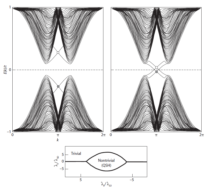
Figure 9.1. Energy bands for a one-dimensional zigzag strip in the (a) QSH phase \(\lambda_{v}=0.1 t\) and (b) the insulating phase \(\lambda_{v}=0.4 t\). In both cases \(\lambda_{\text {so }}=0.06 t\) and \(\lambda_{R}=0.05 t\). The edge states on a given edge cross at \(k a=\pi\). The inset show the phase diagram as a function of \(\lambda_{v}\) and \(\lambda_{R}\) for \(0<\lambda\) so \(\ll t\)
Each edge has a pair of counterpropagating edge modes, which cross at some \(T\) -invariant point. This crossing is protected by \(T\) symmetry. As long as time reversal is preserved, every k-point in the system must have a \(T\) orthogonal counterpart at \(- k\). The \(T\) -invariant points must each have two states, by Kramers' theorem. That means the gap can never open for a single pair of counterpropagating modes. For every edge in the system, we will observe a pair of edge modes. The dispersions of different edges can cross at some non- \(T\) -invariant point, as in fig. \(9.1\) (a), but the matrix elements coupling these points are zero because they have to fully traverse the system length. Hence there is no one-body, \(T\) -invariant local perturbation term that can couple the two branches of a single pair of edge modes. The situation could not be more different for an even number of a pair of edge modes on the same edge. In this case, the modes can open gaps at the intersection points between the twopairs (which can be away from a \(T\) -invariant \(BZ\) point). \(T\) does not protect that gap opening because a gap opening at \(k \neq 0\) can be accompanied by another gap opening at \(-k \neq 0\), which can cancel the \(T\) breaking of the first. Different pairs of the two modes scatter between themselves and can open a gap because the matrix elements are on the same edge.
If \(S_{z}\) is a good quantum number, threading a flux through the system takes one spin from the left edge, \(A\), to the right edge, \(B\), and takes spin \(\downarrow\) from edge \(B\) to edge \(A\). Hence the system pumps quantized spin and has a quantized spin-Hall conductance of 2 (in units of \(\left.e^{2} / h\right)\). When \(S_{z}\) is not a good quantum number, the system does not have quantized spinHall conductance, but spin still gets pumped. We will see in chapter 10 that the system has a quantized TR polarization.
9.3 First Topological Insulator: Mercury Telluride Quantum Wells
Unfortunately, the initial proposal [4] of a topological insulator in graphene was shown to be experimentally hard to achieve \([42,43]\) : the gap openedby the spin-orbit interaction turns out to be extremely small, of the order of \(10^{-3}\) meV. From theoretical investigations of the typeIII HgTe semiconductor quantum wells, it was then shown [7] that the topological insulating state should be realized in the "inverted" regime, where the quantum-well thickness \(d_{Q W}\) is greater than a certain critical thickness \(d_{c}\). The mechanism by which the topological insulator comes about, band inversion, was later shown to be generic [9]. Most topological insulators discovered today come about through band inversion.
9.3.1 Inverted Quantum Wells
We first try to give a general overview of the band structure for inverted quantum wells. The form of the Hamiltonian from which we will show the existence of a topological insulator in these quantum wells can be determined from symmetry requirements only, at least when expanded close to the \(\Gamma\) -point \(( k =0)\). The central feature of the type-III quantum wells is band inversion: the barrier material such as cadmium telluride (CdTe) has a normal semiconductor bandprogression (similar to, say, gallium arsenide (GaAs)), with the \(\Gamma_{6} s\) -type band lying above the \(\Gamma_{8} p\) -type band and the well material HgTe having an inverted band progression whereby the \(s\) -type \(\Gamma_{6}\) band lies below the \(p\) -type \(\Gamma_{8}\) band. The \(\Gamma_{8}\) band is an angular momentum \(\frac{3}{2}\) band (made out of the angular momentum 1 of the \(p\) -orbitals and electron spin \(\frac{1}{2}\), which are coupled by spin-orbit coupling), and its projections on the \(S_{z}\) quantum number are \(\pm \frac{1}{2}\) and \(\pm \frac{3}{2} .\) The \(\Gamma_{6}\) band is a spin- \(\frac{1}{2}\) band. In both these materials, the gap is the smallest near the -point in the BZ (fig.9.2). Therefore, we shall restrict ourselves to a six-band model and start with the following six basic atomic states per unit cell combined into a six-component spinor: \[ \Psi=\left(\left|\Gamma_{6}, \frac{1}{2}\right\rangle,\left|\Gamma_{6},-\frac{1}{2}\right\rangle,\left|\Gamma_{8}, \frac{3}{2}\right\rangle,\left|\Gamma_{8}, \frac{1}{2}\right\rangle,\left|\Gamma_{8},-\frac{1}{2}\right\rangle\left|\Gamma_{8},-\frac{3}{2}\right\rangle\right) \] This would be the band labeling in a three-dimensional material. In quantum wells grown in the [001] direction, the cubic, or spherical symmetry, is broken down to the axial rotation symmetry in the plane. These six bands combine to form the spin \(\uparrow\) and spin- \(\downarrow(\pm)\) states of three quantum well subbands that have been labeled \(E 1, H 1, L 1\) in the literature \([44]\). The \(L 1\) subband is separated from the other two [44], and we neglect it, leaving an effective four-band model for thin quantum wells. At the \(\Gamma\) -point with in-plane momentum \(k_{1}=0, m_{J}\) is still a good quantum number. At this point the \(\left|E 1, m_{j}\right\rangle\) quantum-well subband state is formed from the linear combination of the \(\left|\Gamma_{6}, m_{J}=\pm \frac{1}{2}\right\rangle\) and the \(\left|\Gamma_{8}, m_{I}=\pm \frac{1}{2}\right\rangle\) states, whereas the \(\left|H 1, m_{I}\right\rangle\) quantum-well subband state is formed from the \(\left|\Gamma_{8}, m_{j}=\pm \frac{3}{2}\right\rangle\) states. Away from the \(\Gamma\) -point, the \(E 1\) and the \(H 1\) states can mix. Because the \(\left|\Gamma_{6}, m_{J}=\pm \frac{1}{2}\right\rangle\) state has opposite parity from the \(\left|\Gamma_{8}, m_{I}=\pm \frac{3}{2}\right\rangle\) state under 2 -D spatial reflection, the coupling matrix element between these two states must be an odd function of the in-plane momentum \(k\). This is also true by considering the fact that the coupling between an \(m_{J}=\frac{3}{2}\) state and an \(m_{J}=\frac{1}{2}\) state has to be an \(\Delta L_{z}=1\) coupling. The inplane momentum \(k_{+}=k_{x}+i k_{y}\) provides that coupling. From these symmetry considerations, we deduce the general form of the effective Hamiltonian for the \(E 1\) and the \(H 1\) states, expressed in the basis of \(\left|E 1, m_{I}=\frac{1}{2}\right\rangle,\left|H 1, m_{I}=\frac{3}{2}\right\rangle\) and \(\left|E 1, m_{I}=-\frac{1}{2}\right\rangle,\left|H 1, m_{I}=-\frac{3}{2}\right\rangle\) : \[ H_{\text {eff }}\left(k_{x}, k_{y}\right)=\left(\begin{array}{cc} H( k ) & 0 \\ 0 & H^{*}(- k ) \end{array}\right), \quad H( k )=\epsilon( k )+d_{i}( k ) \sigma_{i} \] where \(\sigma_{i}\) are the Pauli matrices. The form of \(H^{*}(- k )\) in the lower block is determined from TR symmetry (as we will see in chap. 12) and \(H^{*}(- k )\) is unitarily equivalent to \(H^{*}( k )\) for this system. If inversion symmetry and axial symmetry around the growth axis are not broken, then the interblock matrix elements vanish, as presented. In real HgTe, however, inversion symmetry is softly broken, and off-diagonal terms are present. However, because they are small and do not close the bandgap, we can analyze the physics in the absence of these terms and argue by adiabatic continuity that the same topological physics remains valid when the inversion breaking-terms are added.
We see that, to the lowest order in \(k\), the Hamiltonian matrix decomposes into \(2 \times 2\) blocks, for each spin \(\uparrow, \downarrow .\) The preceding Hamiltonian has more symmetry than only inversion symmetry \(-\) in fact it has \(U(1) \times U(1)\) symmetry, which are the two quantum Hall effects in the two spins separately. From the symmetry arguments given before, we deduce that \(d_{3}( k )\) is an even function of \(k\), whereas \(d_{1}( k )\) and \(d_{2}( k )\) are odd functions of \(k-\) they are \(L_{z}=1\) terms. Therefore, we can generally expand them in the following form: \[ \begin{array}{c} d_{1}+i d_{2}=A\left(k_{x}+i k_{y}\right) \equiv A k_{+} \\ d_{3}=M-B\left(k_{x}^{2}+k_{y}^{2}\right), \quad \epsilon_{k}=C-D\left(k_{x}^{2}+k_{y}^{2}\right) \end{array} \] where the constants \(A, M, B, C\), and \(D\) can be obtained from a first-principle (or perturbative) calculation.Their approximate values are given in Table \(9.1\), \[ \begin{array}{|c|c|c|c|c|c|} \hline \hline d( nm ) & A( eV ) & B( eV ) & C( eV ) & D( eV ) & M( eV ) \\ \hline 5.8 & -3.62 & -18.0 & -0.0180 & -0.594 & 0.00922 \\ \hline 7.0 & -3.42 & -16.9 & -0.0263 & 0.514 & -0.00686 \\ \hline \end{array} \]
Parameters for \(Hg _{0.32} Cd _{0.68}\) Te/HgTe quantum wells.
and the band dispersion is shown in fig. \(9.2\)
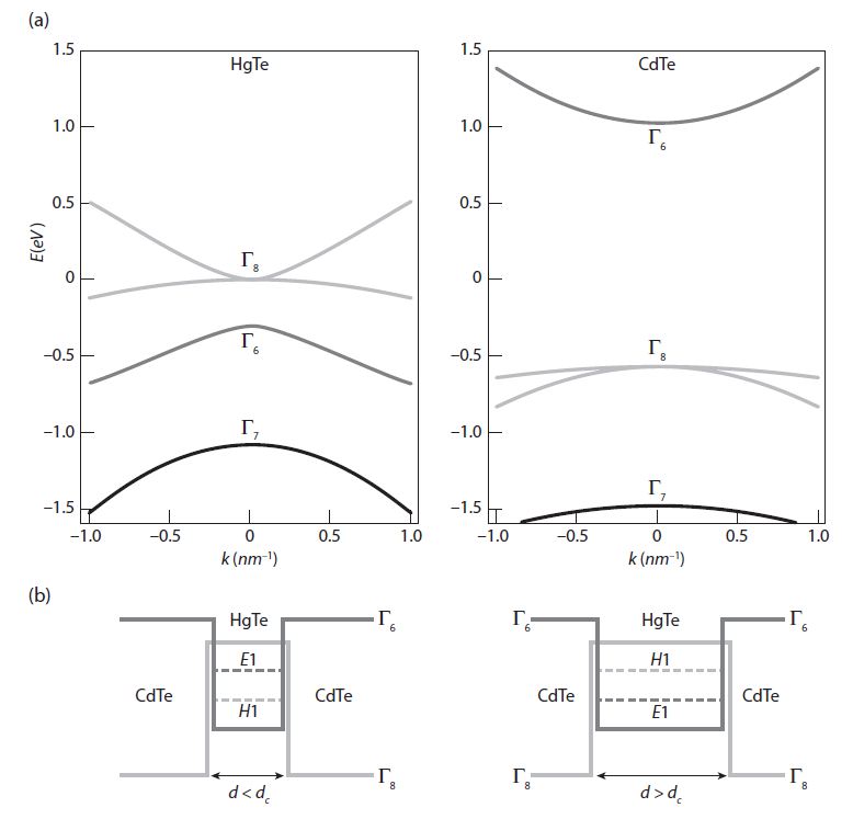
Figure 9.2. (A) Bulk energy bands of HgTe and CdTe near the \(\Gamma\) point. (B) The CdTe/HgTe/CdTe quantum well in the normal regime \(E 1>H 1\) with \(d<d_{c}\) and in the inverted regime \(H 1>E 1\) with \(d>d_{c} .\) In this, and all subsequent figures, \(\Gamma_{8} / H 1\) \(\left(\Gamma_{6} / E 1\right)\) symmetry is correlated with the color red (blue).
The Hamiltonian in the \((2 \times 2)\) subspace therefore takes the form of the \((2+1)\) D Dirac Hamiltonian, plus an \(\epsilon(k)\) term, which drops out in the quantum Hall response. We discard this term from now on. Within each \(2 \times 2\) subblock, the Hamiltonian has the Hall conductance \[ \sigma_{x y}=-\frac{1}{8 \pi^{2}} \iint d k_{x} d k_{y} \hat{ d } \cdot\left(\partial_{ x } \hat{ d } \times \partial_{y} \hat{ d },\right) \] in units of \(e^{2} / h\), where \(\hat{ d }\) denotes the unit \(\hat{d}_{i}(k)\) vector introduced in the Hamiltonian (eq (9.37)). Although we are in the continuum, the Dirac Hamiltonian is regularized properly by the presence of the \(k^{2}\) terms in the \(d_{3}( k )\) term. However, if the \(k^{2}\) terms were not present, the Dirac Hamiltonian would have Hall conductance \(\frac{\operatorname{sig}(M)}{2} .\) The presence of the quadratic terms renders the Hall conductance an integer that is based on whether or not the vector \(\hat{d}_{3}\) winds from \(k =0\) to \(k =\infty\) from the north to the south pole of the \(S^{2}\) sphere. If \(M / B>0\), then it is clear that \(d_{3}\) points to one pole at \(k =0\) and to another at \(k =\infty\). This is the continuum regularization of a Dirac Hamiltonian and will be, for example, used in the \(p+i p\) model of a topological superconductor in chapter \(16 .\) The most important quantity in the Hamiltonian is the mass, or gap parameter, \(M\), which is the energy difference between the \(E 1\) and \(H 1\) levels at the \(\Gamma\) -point. The overall constant \(C\) sets the zero of energy to be the top of the valence band of bulk HgTe. In a quantum-well geometry, the band inversion in HgTe necessarily leads to a level crossing at some critical thickness \(d_{c}\) of the HgTe layer. For thickness \(d<d_{c}\), i.e., for a thin HgTe layer, the quantum well is in the "normal" regime, where the CdTe is predominant; hence, the band energies at the \(\Gamma\) -point satisfy \(E\left(\Gamma_{6}\right)>E\left(\Gamma_{8}\right)\). For \(d>d_{c}\) the HgTe layer is thick and the well is in the inverted regime where HgTe dominates and \(E\left(\Gamma_{6}\right)<E\left(\Gamma_{8}\right) .\) As we vary the thickness of the well, the \(E 1\) and \(H 1\) bands must, therefore, cross at some \(d_{c}\), and the gap parameter \(M\) changes sign between the two sides of the transition (fig. \(9.3\) ). The form of the effective Dirac Hamiltonian and the sign change of \(M\) at \(d=d_{c}\) for the HgTe/CdTe quantum wells deduced previously from general arguments is sufficient to conclude the existence of the quantum-spin Hall (QSH) state in this system. As we change the quantum-well thickness \(d\) across \(d_{c}, M\) changes sign, and the gap closes at the \(\Gamma\) point leading to a vanishing \(d_{i}( k =0)\) vector at the transition point \(d=d_{c}\). The sign change of \(M\) leads to a well-defined change of the Hall conductance \(\Delta \sigma_{x y}=1\) across the transition. So far, we have discussed only one \(2 \times 2\) block of the effective Hamiltonian, \(H .\) General TR symmetry dictates that \(\sigma_{x y}(H)=-\sigma_{x y}\left(H^{*}\right) ;\) therefore, the total charge Hall conductance vanishes, whereas the spin Hall conductance, given by the difference between the two blocks, is finite and is given by \(\Delta \sigma_{x y}^{(s)}=2\) (in units of \(\left.e^{2} / h\right)\). From the general relationship between the quantized Hall conductance and the number of edge states, we conclude that the two sides of the phase transition at \(d=d_{c}\) must differ in the number of pairs of helical edge states by 1 . Thus, one side of the transition must be \(Z_{2}\) odd and topologically distinct from a fully gapped conventional insulator. To find out which side must be topologically nontrivial, we have to compute the value of \(M / B\), but the overwhelming evidence points to the inverted side being topologically nontrivial. Indeed, in the inverted gap regime where \(\frac{M}{2 B}=2.02 \times 10^{-4}\) at \(7.0 nm\) and not in the normal regime (where \(\frac{M}{2 B}<0\) ), and the inverted case is the topologically nontrivial regime supporting a QSH state. Figure \(9.3\) shows the energies of both the \(E 1\) and \(H 1\) bands at \(k_{\|}=0\) as a function of quantum-well thickness \(d\) obtained from our analytical solutions. At \(d=d_{c} \sim 6.4 nm\), these bands cross.
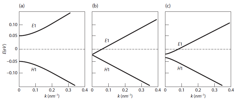
Figure 9.3. (A) Energy (eV) of \(E 1\) and \(H 1\) bands at \(k_{\|}=0\) versus. quantum-well thickness \(d\) (A). (b) Energy dispersion relations \(E\left(k_{x}, k_{y}\right)\) of the \(E 1, H 1\) subbands at \(4.0 nm , 6.35 nm\) and \(7.0 nm\) from left to right. Colored shading indicates the symmetry type of band at that \(k\) -point. Places where the cones are more red (blue) indicates that the dominant states are \(H 1(E 1)\) states at that point. Purple shading is a region where the states are more evenly mixed in character. For \(4.0 nm\) the lower (upper) band is dominantly \(H 1(E 1)\). At \(6.35 nm\) the bands are evenly mixed near the band crossing and retain their \(d<d_{c}\) behavior moving further out in \(k\) -space. At \(d=7.0 nm\), the regions near \(k_{\|}=0\) have flipped their character but eventually revert back to the \(d<d_{c}\) further out in \(k\) -space. Only this dispersion shows the meron structure. (c) Schematic meron configurations representing the \(d_{i}( k )\) vector near the point \(\Gamma\). The shading of the merons has the same meaning as the preceding dispersion relations. The change in meron number across the transition is exactly equal to 1 , leading to a quantum jump of the spin Hall conductance \(\Delta \sigma_{x y}^{(s)}=2 e^{2} / h\). All plots are for \(Hg _{0.32} Cd _{0.68}\) Te/HgTe quantum wells.
9.4 Experimental Detection of the Quantum Spin Hall State
We now discuss the experimental detection of the QSH state. We want to focus only on purely electrical measurements because spin measurements are difficult to achieve. By sweeping the gate voltage, we can measure the two-terminal conductance \(G_{L R}\) from the \(p\) -doped to bulkinsulating to \(n\) -doped regime(figs. \(9.4\) and \(9.5\) ). In the bulk-insulating regime, \(G_{L R}\) vanishes at low temperatures for a normal insulator at \(d<d_{c}\), whereas \(G_{L R}\) approaches a value close to \(\frac{2 e^{2}}{h}\) for \(d>d_{c}\) and for samples shorter than the mean free inelastic scattering path. This has been observed in a remarkable experiment performed at the University of Wurzburg [8].
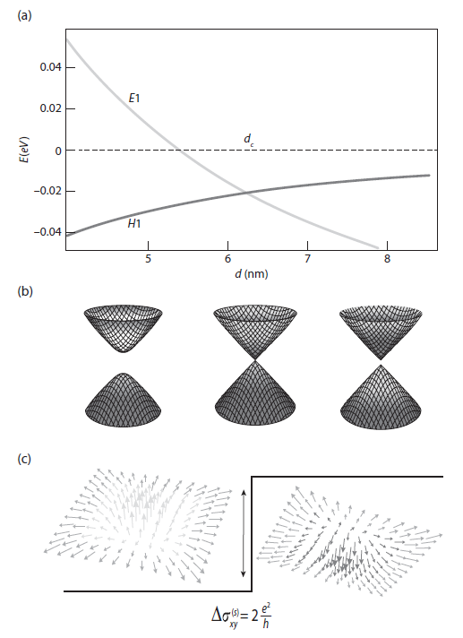
Figure 9.4. (a) Experimental setup on a six-terminal Hall bar showing pairs of edge states with spin-up (spin-down) states given in green (purple). (b) A two-terminal measurement on a Hall bar would give \(G_{\angle R}\) close to \(2 e^{2} / h\) contact conductance on the QSH side of the transition and zero on the insulating side. In a six-terminal measurement, the longitudinal voltage drops \(\mu_{2}-\mu_{1}\) and \(\mu_{4}-\mu_{3}\) vanish on the QSH side with a power law as the zero-temperature limit is approached. The spin Hall conductance \(\sigma_{x y}^{(s)}\) has a plateau with the value close to \(2\left(e^{2} / h\right)\).
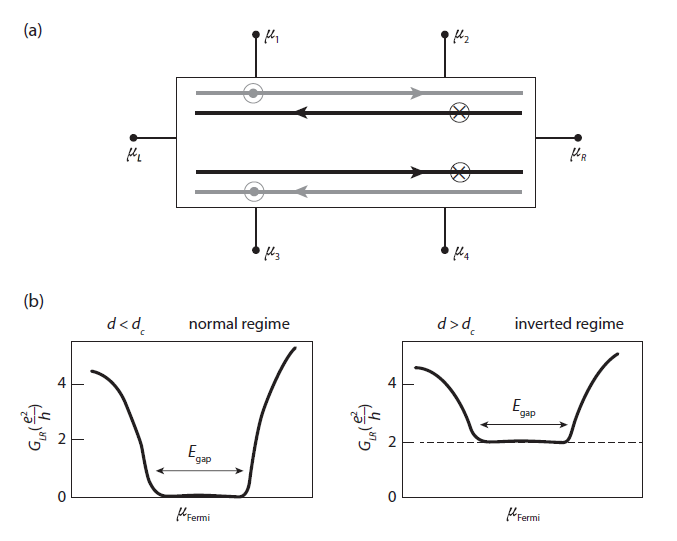
Figure 9.5. Dispersion relations for the \(E 1\) and \(H 1\) subbands for (a) \(d=4.0 nm\) and (b) \(d=6.35 nm\), and (c) \(d=7.0 nm\).
Strikingly, in a six-terminal measurement, the QSH state would exhibit vanishing electric voltage drop between the terminals \(\mu_{1}\) and \(\mu_{2}\) and between \(\mu_{3}\) and \(\mu_{4}\) in the zero-temperature limit and in the presence of a finite electric current between the \(L\) and \(R\) terminals. In other words, longitudinal resistance should vanish in the zero-temperature limit with a powerlaw dependence, over distances larger than the mean free path. Because of the absence of backscattering, in the absence of leads along the path between source and drain, the helical edge currents flow without dissipation, and the voltage drop occurs only at the drain side of the contact [45]. Finally, a spin filtered measurement can be used to determine the spin Hall conductance \(\sigma_{x x}^{(s)}\), although we expect this to be much more experimentally challenging. Numerical calculations [46] show that it should take a value close to \(\sigma_{x y}^{(s)}=2\left(e^{2} / h\right)\). This experiment has not yet been performed.