[TOC]
参考
- 《Topological Insulators and Topological Superconductors》 - B. Andrei Bernevig
- Chapter-8 Simple Models for the Chern Insulator
- Chapter-9
Chapter-8 Simple Models for the Chern Insulator
We are now well prepared to discuss the simplest model of a topological insulator, the Chern insulator on the square lattice.
- Even though, historically, the first model of a Chern insulator was introduced by Haldane on the hexagonal lattice (which we study after the square-lattice call), a Chern insulator model on the square lattice is easier to introduce and understand.
- Before we do that, however, we must first understand the behavior of Dirac fermions upon opening a gap in their spectrum.
- The previous chapter focused on how to keep the Dirac fermions gapless. This chapter focuses on how to make them massive and the implications of making them massive.
- We will learn that massive Dirac fermions in the continuum exhibit a half-integer quantum Hall effect, and we will tie up some loose ends with regard to prior cryptic statements about smooth gauge, Stokes' theorem, and others.
- We will then show that Dirac fermions are very useful in obtaining the Hall conductance of systems that undergo a gap-closing-and-reopening transition.
8.1 Dirac Fermions and the Breaking of Time-Reversal Symmetry
In two dimensions, the model for a continuum Dirac fermion is a variant of the general two-level Hamiltonian: \[ h( k )=\sum_{i} d_{i}( k ) \sigma_{i} \] where
- \(d_{1}=k_{x}, d_{2}=k_{y}\) up to a rotation.
If \(d_{3}=0\), then the Hamiltonian is gapless, whereas if \(d_{3}=M\) is a constant, then the Dirac fermion is gapped. We now show that when the \(\sigma\) matrices correspond to spin, the first case maintains time reversal, whereas the latter breaks it. Notice that here the momentum \(k\) is a continuum variable lying in the infinite Euclidean plane.
8.1.1 When the Matrices \(\sigma\) Correspond to Real Spin
If the Dirac equation matrix structure comes from real spin, then we have \(T=-i \sigma_{y} K\), and we know that all three matrices \(\sigma_{i}\) are odd under time reversal. Then \[ T h( k ) T^{-1}=-d_{i}( k ) \sigma_{i}=-k_{x} \sigma_{x}-k_{y} \sigma_{y}-M \sigma_{z} \] If \(T\) is preserved, then the preceding should equal \(h(- k )=-k_{x} \sigma_{x}-k_{y} \sigma_{y}+M \sigma_{z} .\) This is possible only when \(M=0\), i.e., when the system is gapless. Generalization to any \(d_{i}( k )\) shows that if time reversal is to be preserved, then \[ \operatorname{Th}( k ) T^{-1}=-d_{i}( k ) \sigma_{i}=h(- k )=d_{i}(- k ) \sigma_{i} ; \rightarrow \quad d_{i}(- k )=-d_{i}( k ) \] Notice that the conditions on the vector \(d_{i}( k )\) are different from the graphene case, in which the matrices \(\sigma\) were not meant to represent the spin of the particle. At special points that are invariant (modulo a reciprocal lattice vector) under time reversal \[ k _{\text {special }}=(0,0),(0, \pi),(\pi, 0),(\pi, \pi)=- k _{\text {special }}= G / 2 \] we find that \[ d_{i}( G / 2)=-d_{i}(- G / 2)=-d_{i}( G / 2)=0 \] for each \(i\); hence the system must be gapless. This can, of course, be more simply understood by just drawing the picture of a gapped Dirac fermion and seeing that the state \(k=0\) does not have a Kramers' pair. Because we are working in a spin- \(\frac{1}{2}\) system, this necessarily implies the breaking of time reversal.
8.1.2 When the Matrices \(\sigma\) Correspond to Isospin
In this case, \(T^{2}=1\) and the preceding condition for TR symmetry changes to \(h^{*}( k )=h(- k )\). This implies \(d_{1}( k )=d_{1}(- k ), d_{2}( k )=-d_{2}(- k )\), and \(d_{3}( k )=d_{3}(- k )\). It then turns out that to maintain time reversal, we need \(d_{1}, d_{3}\) to be even in \(k\) but \(d_{2}\) to be odd. Of course, in this case the Chern number has to vanish.
8.2 Explicit Berry Potential of a Two-Level System
Let us now try to explicitly obtain the Berry potential and Berry field strength for a two-level system. The energies of the Hamiltonian in equation (8.1) \(h(k)=\sum_{i} d_{i}(k) \sigma_{i}\) , \[ E_{\pm}=\pm \sqrt{d_{1}^{2}+d_{2}^{2}+d_{3}^{2}} \equiv \pm d \] The eigenstates of the Hamiltonian are \[ \psi_{E_{+}}=\frac{1}{\sqrt{2 d\left(d+d_{3}\right)}}\left(\begin{array}{c} d_{3}+d \\ d_{1}-i d_{2} \end{array}\right), \quad \psi_{E_{-}}=\frac{1}{\sqrt{2 d\left(d-d_{3}\right)}}\left(\begin{array}{c} d_{3}-d \\ d_{1}-i d_{2} \end{array}\right) \] which are properly normalized and orthogonal. We try to compute the Berry connection: \[ A_{i}( k )=i\left\langle\psi_{E_{-}}\left|\partial_{k_{i}}\right| \psi_{E_{-}}\right\rangle=\frac{-1}{2 d\left(d+d_{3}\right)}\left(d_{2} \partial_{i} d_{1}-d_{1} \partial_{i} d_{2}\right) \] We can then obtain the Berry curvature [40]: \[ F_{i j}=\frac{1}{2 d^{3}} \epsilon_{a b c} d_{a} \partial_{i} d_{b} \partial_{j} d_{c}=\frac{1}{2} \epsilon_{a b c} \hat{d}_{a} \partial_{i} \hat{d}_{b} \partial_{j} \hat{d}_{c} \] where
- \(\hat{d}_{a}=d_{a} / d\).
We notice that the field strength is the Jacobian of the map \(k \rightarrow d / d\), which is a map between the base manifold-a 2-D momentum space-and the target manifolda 2-D sphere \(S^{2}\) -given by the equation \(d^{2}=1\). When integrated over the base manifold, the Jacobian counts the winding number of the map, which is always an integer, the Chern number.
8.2.1 Berry Phase of a Continuum Dirac Hamiltonian
The 2-D Dirac Hamiltonian, in the continuum, corresponds to the case \(d_{3}=m, d_{1}=k_{x}, d_{2}=k_{y}\). Let us now compute the vector potential by plugging, values into this formula: \[ A_{x}=\frac{-k_{y}}{2 \sqrt{k^{2}+m^{2}}\left(\sqrt{k^{2}+m^{2}}+m\right)}, \quad A_{y}=\frac{k_{x}}{2 \sqrt{k^{2}+m^{2}}\left(\sqrt{k^{2}+m^{2}}+m\right)} . \] Let us assume we are at finite chemical potential \(\mu\) larger than the mass gap \(m\), which endows us with a Fermi surface. Note that although we did not implicitly put the chemical potential
into the Hamiltonian, the Berry vector potential remains unchanged because the chemical potential is a diagonal identity matrix term and the eigenstates are not changed by diagonal terms. If the eigenstates are unchanged, the Berry potential is unchanged as well. We then would like to integrate the Berry curvature over the Fermi surface, which is an azimuthal integration over the angle at a momentum \(k_{F}=\sqrt{\mu^{2}-m^{2}}\) (note that we are using \(\hbar=1\) ). Hence, for the integral of the Berry potential over the Fermi surface, we obtain \[ \begin{aligned} \int_{\text {Fermi surface }} d k \cdot A =&\int_{0}^{2 \pi} k_{F} d \theta A_{\theta} \\=&\int_{0}^{2 \pi} k_{F} d \theta\left(A_{y} \frac{k_{x}}{k_{F}}-A_{x} \frac{k_{y}}{k_{F}}\right) \\=&\int_{0}^{2 \pi} \frac{k_{F}^{2}}{2 \sqrt{k_{F}^{2}+m^{2}}\left(\sqrt{k_{F}^{2}+m^{2}}+m\right)} d \theta \\=&\left.\pi \frac{k_{F}^{2}}{\sqrt{k_{F}^{2}+m^{2}}\left(\sqrt{k_{F}^{2}+m^{2}}+m\right)} \approx\right|_{m / k_{F}<<1} \\=&\pi-\pi \frac{m}{k_{F}} \end{aligned} \] Notice that the Berry phase at the TR-invariant (gapless) \(m=0\) point is \(\pi\); this be can easily understood because \(\pi\) is the only value (besides 0 ) that is TR invariant (modulo \(2 \pi\) ). When time reversal is broken, the Berry phase around the Fermi surface picks up a contribution proportional to the ratio between the gap and the Fermi momentum-so if the Fermi level is really high, corresponding to large doping, then the Berry phase can be again very close to (but not equal) \(\pi\), even though the time reversal is broken.
8.2.2 The Berry Phase for a Generic Dirac Hamiltonian in Two Dimensions
In the previous derivation of the Berry phase, we have assumed rotational invariance. However, around a degeneracy point or band, crossing in two-dimensions, we have the following general form for the Hamiltonian: \[ h( k )=k_{i} A _{i j} \sigma_{j}, \] with \(A _{i j}\) a \(2 \times 2\) matrix. We have neglected a possible diagonal term proportional to the identity matrix because it does not influence the eigenstates and, hence, does not enter the Berry phase. The eigenvalue of the Hamiltonian \(d=\sqrt{\left( A _{1 i} k_{i}\right)^{2}+\left( A _{2 i} k_{i}\right)^{2}}\) and the Berry potential is \[ A_{i}( k )=-\frac{1}{2 d^{2}}\left( A _{2 j} k_{j} A _{1 i}- A _{1 j} k_{j} A _{2 i}\right) \] We want to compute the Berry phase over the Fermi surface (see fig. 8.1), but, in general, the Fermi surface can be anisotropic. However, we have \(A_{i} d k_{i}=A_{\phi} k(\phi) d \phi\) because an infinitesimal variation \(d k =k(\phi) d \phi \hat{1}_{\phi}\) on the Fermi surface. Here, \(\hat{1}_{\phi}\) is the unit vector tangential to a surface of equal energy in \(k\) -space. We have that \[ A_{\phi}=A_{y} \frac{k_{x}}{k}-A_{x} \frac{k_{y}}{k} \] so the Berry phase is \[ \int_{0}^{2 \pi} d \phi\left(A_{y} k_{x}-A_{x} k_{y}\right)=\int_{0}^{2 \pi} d \phi \frac{1}{2 d^{2}} k^{2} \operatorname{Det} A \] which, upon substituting for \(d\) and using the integral \[ \int_{0}^{2 \pi} d \phi \frac{1}{a \cos (\phi)^{2}+b \sin (\phi)^{2}+c \cos (\phi) \sin (\phi)}=\frac{4 \pi}{\sqrt{4 a b-c^{2}}} \] valid as long as \(c^{2}<4 a b\), which is the condition of not having nodal lines, brings us to a nice expression for the Berry phase: \[ \int_{\text {Fermi surface }} d k \cdot A =\pi \cdot \operatorname{sign}(\operatorname{Det} A ) . \] ### 8.2.3 Hall Conductivity of a Dirac Fermion in the Continuum
The Berry curvature, necessary for the Chern number, vanishes on a lattice if you have time reversal. The Dirac fermion in the continuum does not have a lattice by definition, but the same theorem applies. This can be clearly seen from the form of the Berry curvature, which needs all three Pauli matrices to enter. For the continuum Dirac Hamiltonian, using equation (8.7) we have \[ F_{x y}=\frac{1}{2\left(m^{2}+k^{2}\right)^{3 / 2}} m \] In contrast to the computation of the Berry phase, we now put the chemical potential in the gap \((|\mu|<m)\) and integrate the Berry curvature over the occupied states (this is the Berry curvature of the occupied band): \[ \begin{aligned} \sigma_{x y}=&\frac{e^{2}}{h} \frac{1}{2 \pi} \int d^{2} k F_{x y} \\=&\frac{e^{2}}{h} \frac{m}{4} \int_{0}^{\infty} d x \frac{1}{\left(m^{2}+x\right)^{3 / 2}} \\=&\frac{e^{2}}{h} \frac{\operatorname{sign}(m)}{2} . \end{aligned} \] We have arrived at the notable result that massive 2-D Dirac fermions have a Hall conductance equal to one-half times the sign of their mass. This statement is puzzling because the Hall conductance, equal to the Chern (winding) number of the filled band, has to be an integer. This is true, but only if the problem is on a lattice-in this case, the reason we get one-half is because the Dirac fermion is in the continuum and has not been regularized properly. The bands of the continuum Dirac fermion do not have a bandwidth. The Hall conductance equals the Chern number and is an integer only if the base manifold (the BZ) is compact. In the continuum, the momentum runs over a noncompact manifold (the infinite Euclidean plane), and this does not apply.
How does having a lattice fix things? If we are on a lattice, the bands, which in the case of the Dirac fermion have infinite bandwidth (because the dispersion is \(\left.\pm \sqrt{k^{2}+m^{2}}\right)\), must bend down due to the fact that the problem has a finite bandwidth. At the points where the bands bend down (roughly), we will get another half a quantum of Hall conductance. These highenergy fermions, which contribute to conductances, are called spectator fermions. The moral of the story is that we cannot determine the full Hall conductance of a filled band by analyzing the physics of only a small part of the band. For example, in an insulator, the vicinity of the \(k\) -space point where the gap is the smallest can be modeled by a Dirac Hamiltonian. However, due to the presence of the spectator fermions just mentioned, we cannot calculate the Hall conductance of the filled lattice band just by looking at the points where the gap is the smallest and then performing the Dirac computation. The reason is that we might have some higherenergy modes that can add or subtract half-values. However, the change in Hall conductance upon closing or reopening the gap can be determined by focusing only on the vicinity of the point where the transition happens. Generically, a gap-closing-and-opening transition has to happen by varying a parameter, the mass of the Dirac fermion \(m\). If we go from \(m\) negative to \(m\) positive (and, in the process, close the gap and reopen it), then we get the Hall conductance to change by 1 . If we knew the value of the Hall conductance before the gap-closing transition, we would be able to find the value of the Hall conductance after closing and reopening the gap.
8.3 Skyrmion Number and the Lattice Chern Insulator
In the previous subsection, we saw that the Dirac fermions are nontrivial physical systems. So far we have looked at the Dirac Hamiltonian in the continuum, but it seems reasonable to assume that their lattice generalization will also yield nontrivial physics. We now would like to make the simplest lattice generalization of the continuum Dirac Hamiltonian: instead of \(k_{x}, k_{y}\), we generalize this to \(\sin \left(k_{x}\right), \sin \left(k_{y}\right)\), whereas the mass of the Dirac Hamiltonian can be generalized to \(2+M-\cos \left(k_{x}\right)-\cos \left(k_{y}\right)\). This lattice generalization becomes the continuum Dirac Hamiltonian for momentum close to \(k=0 .\) As we have already shown, the Hamiltonian for an insulator (spinless) must contain two bands. The lattice generalization of the Dirac Hamiltonian is, hence, an orbital model with two orbitals per site, one of \(s\) -type and one of \(p\) -type (or, more generally, orbitals of different parity). The coupling between the \(s\) and \(p\) orbitals thus must necessarily be an angular-momentum \(L=1\) coupling; hence, the lowest-order coupling is linear in \(k\left(\sin \left(k_{x}\right)+i \sin \left(k_{y}\right)\right)\). We also add intraorbital dispersions \(2-\cos \left(k_{x}\right)-\cos \left(k_{y}\right)\) because they are allowed by symmetry. Hence, to the lowest-order in Fourier modes, the Hamiltonian necessarily must look like \[ H=\sin \left(k_{x}\right) \sigma_{x}+\sin \left(k_{y}\right) \sigma_{y}+B\left(2+M-\cos \left(k_{x}\right)-\cos \left(k_{y}\right)\right) \sigma_{z} \] This Hamiltonian is fully gapped except at several values of \(M\) : at \(M=0\), it is gapless at \(\left(k_{x}, k_{y}\right)=(0,0) ;\) at \(M=-2\), it is gapless at \(\left(k_{x}, k_{y}\right)=(\pi, 0),(0, \pi)\) and at \(M=-4\), it is gapless at \(\left(k_{x}, k_{y}\right)=(\pi, \pi) .\) By adiabatic continuity, as long as the Hamiltonian is gapped and the gap does not close, it remains in the same topological phase. By varying the parameter \(M\), the model has phase transitions and different topological properties, which we now investigate.
8.3.1 \(M>0\) Phase and \(M<-4\) Phase
In these two regimes, the Hamiltonian is fully gapped and the Chern number is zero, per direct computation. This can be explained in different ways. We can do a direct numerical computation using the Jacobian curvature, but this would not be very physically revealing. The most physically revealing is to realize that both \(M>0\) and \(M<-4\) represent Hamiltonians topologically equivalent to the atomic limit (the limit in which all hoppings are set to zero, as if the lattice constant were infinity). The \(M>0\) regime is topologically the same phase as the phase \(M \rightarrow \infty\), which has trivial (momentum-independent) eigenstates and zero Hall conductance. This is, in fact, an atomic limit, which does not show anything interesting because the energy bands are flat and only on-site energies are important so the wavefunctions are completely localized on the atomic sites. Here, \(M<-4\) is topologically the same as \(M \rightarrow-\infty\), which is also an atomic limit but with the on-site energies reversed from the \(M \rightarrow \infty\) phase.
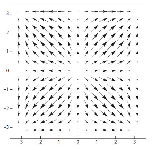
Figure 8.2. Vector plot for the components \(d_{1}(k)=\sin \left(k_{x}\right), d_{2}(k)=\sin \left(k_{y}\right)\) in the Chern insulator, \(e_{s}=M / 2 B\).
Another way of understanding that the Chern number is zero is by seeing that the \(d_{3}\) component of the Hamiltonian does not change sign in the \(BZ\). The Hall conductance is a Jacobian integrated over the whole BZs, which is identical to a skyrmion number of the vector \(\hat{d}_{i} .\) Because \(\sin \left(k_{x}\right)\) and \(\sin \left(k_{y}\right)\) form a vector that looks like figure \(8.2\), we see that to realize a skyrmion, we must look at the component of the \(d_{3}\). The configuration of \(d_{3}\) is ferromagnetic (see fig. 8.3) for the values of \(M\) in this section, and so there is no skyrmion in \(\hat{d}_{i}\) and, hence, no nonzero Hall conductance.
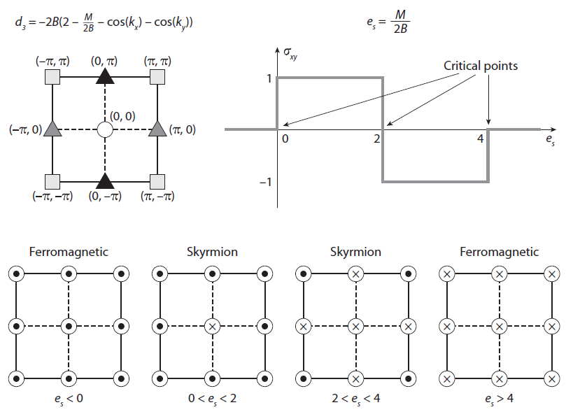
Figure \(8.3 .\) The values of \(d_{2}( k )\) at high-symmetry points in the Brillouin zone and Chern numbers in the Chern insulator. Depending on whether \(d_{3}\) dose or does not change sign in the BZ, we have or do not have skyrmion configurations.
8.3.2 The \(-2<M<0\) Phase
As we decrease \(M\) from the atomic limit \((M=\infty)\), at \(M=0\) the energy gap collapses at the \(\Gamma=(0,0)\) point. All other points remain gapped. Hence, we need to look only for the physics around that particular point if all we care about is the low-energy structure. To find out more information,we would like to obtain the continuum Hamiltonian near that point. We expand to obtain \[ H_{\Gamma+k}=k_{x} \sigma_{x}+k_{y} \sigma_{y}+M \sigma_{z} \] up to linear terms in \(k\). At the gap-closing-and-reopening transition, \(M\) goes from positive to negative, so the change in Hall conductance is \[ \Delta \sigma_{x y}=\frac{1}{2} \operatorname{sign}\left(M_{<0}\right)-\frac{1}{2} \operatorname{sign}\left(M_{>0}\right)=-1 \] Because we know that the initial state had zero Hall conductance, by the preceding arguments, the new state has \[ \sigma_{x y}=-1 \] The Hall conductance corresponds to the skyrmion number in the BZ. For \(-2<M<0\), the configuration of \(d_{3}\) looks like that in the figure \(8.3\) (which was plotted in terms of \(e_{s}=M / B\) ). As such, \(d_{3}<0\) around the \(\Gamma\) point (at exactly that point it is equal to \(M\) ) and then becomes positive at \((\pi, 0),(0, \pi)\), where it becomes equal to \(2+M\). This corresponds to a skyrmion number of \(-1\). This skyrmion number can be understood as the difference between the two meron numbers of the continuum Dirac fermions with \(M>0\) and \(M<0\), which are \(\frac{1}{2}\) and \(-\frac{1}{2}\), respectively (fig. 8.4). The continuum Dirac equation has a meron in it because \(d_{3}=M\) is always in the same direction, but the \(k_{x}, k_{y}\) point away from the origin and, at large values, become dominant over \(d_{3}\), and the vector lies in the plane. However, there is a nontrivial difference between \(M>0\) and \(M<0 .\) The difference between the two Hall conductances of the Dirac fermions (meron numbers) is the skyrmion number equal to \(-1\).
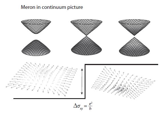
Figure 8.4. The Hall conductance equal to the skyrmion number as the difference between the Dirac equation meron numbers.
8.3.3 The \(-4<M<-2\) Phase
When we decrease \(M\) even further, we reach another phase transition. At \(M=-2\), the gap closes at two points in the BZ: \((\pi, 0)\) and \((0, \pi)\). We can analyze what happens at this phase transition by looking only around those two points. We linearize the Hamiltonian around these points: \[ \begin{array}{l} H_{(\pi, 0)+ k }=-k_{x} \sigma_{x}+k_{y} \sigma_{y}+(2+M) \sigma_{z} \\ H_{(0, \pi)+ k }=k_{x} \sigma_{x}-k_{y} \sigma_{y}+(2+M) \sigma_{z} \end{array} \] and we can see that the Hall conductivity of each of these Dirac Hamiltonians is \[ \sigma_{x y}=-\operatorname{sign} \frac{1}{2}(2+M) \] The reason for the minus sign in front of the Hall conductance is the fact that there is now a minus sign in front of either \(\sigma_{x}\) or \(\sigma_{y}\), respectively, for the two Hamiltonians in vicinity of \((\pi, 0)\) or \((0, \pi)\). For a generic Hamiltonian \(H=k_{\mu} A_{\mu v} \sigma_{v}\), where in this case \(\mu, v=1,2,3\) and \(k_{\mu}=\left(k_{x}, k_{y}, M\right)-\) the Dirac mass - the Hall conductance is given by half the sign of the determinant of \(A\) : \(\sigma_{x y}=\frac{1}{2} \operatorname{sign}(\operatorname{Det}(A))\). We hence have, for the transition between \(M>-2\) and \(M<-2\), a change in Hall conductance of \[ \Delta \sigma_{x y}=2\left(-\frac{1}{2} \operatorname{sign}(M+2)_{M<-2}-\left(-\frac{1}{2} \operatorname{sign}(M+2)_{M>-2}\right)\right)=2 \] Because the phase before the transition \((M>-2)\) had Hall conductance \(-1\), the new Hall conductance is \[ \sigma_{x y}=-1+2=1 \text { . } \]
8.3.4 Back to the Trivial State for \(M<-4\)
At \(M=-4\), yet another point in the \(BZ\) becomes gapless: \((\pi, \pi)\). Anywhere in between the values of \(M=0,-2,-4\), the model is gapped, as it is easily seen from the dispersion. Around the point \((\pi, \pi)\), the Hamiltonian is \[ H_{(\pi, \pi)+ k }=-k_{x} \sigma_{x}-k_{y} \sigma_{y}+(4+M) \sigma_{z}, \] and the change in Hall conductance between \(M>-4\) and \(M<-4\) is \[ \Delta \sigma_{x y}=\frac{1}{2} \operatorname{sign}(4+M)_{M<-4}-\frac{1}{2} \operatorname{sign}(4+M)_{M>-4}=-1 \] which, when added to the previous Hall conductance, gives \(\sigma_{x y}=0\) for \(M<-4\). We have now obtained the full-phase diagram of our model. For the Hall conductance, see the upper right panel in fig \(8.3\).
8.4 Determinant Formula for the Hall Conductance of a Generic Dirac Hamiltonian
So far, we have obtained the Hall conductance for rotationally invariant Dirac Hamiltonians. We now obtain the Chern number for the generic Dirac Hamiltonian: \[ h( k )=k_{a} A _{a b} \sigma_{b}+M \sigma_{3} \] where \(A _{a b}\) are numbers with \(a, b=1,2\) (in a suitable \(\sigma\) basis) and \(M\) is the Dirac gap. The field strength reads \[ F_{12}=\frac{1}{2 d^{3}} M\left( A _{22} A _{11}- A _{21} A _{12}\right)=\frac{1}{2 d^{3}} \operatorname{MDet}( A ) \] where \(d\) is \(d^{2}=k_{m} k_{i} A _{i j} A _{m j}+M^{2} .\)
Going to polar coordinates \(k_{x}=k \sin (\theta), k_{y}=k \cos (\theta)\) we write the Hall conductance as the integral over the occupied states of the Berry curvature; using the identity \[ \int_{0}^{2 \pi} \frac{d \theta}{\left(\cos (\theta)^{2} A _{1 j} A _{1 j}+\sin (\theta)^{2} A _{2 j} A _{2 j}+2 \sin (\theta) \cos (\theta) A _{1 j} A _{2 j}\right)}=\frac{2 \pi}{|\operatorname{Det}( A )|} \] we have that the Hall conductance equals \[ \sigma_{x y}=\frac{1}{2} \operatorname{sign}(M) \operatorname{sign}(\operatorname{Det}( A )) \] Notice that the Hamiltonian in equation (8.28) is not the most general Dirac Hamiltonian: this would be \(k_{\mu} A _{\mu v} \sigma_{v}\), with \(\mu, v=1,2,3\) and \(k_{3}=M\). The Hall conductance of such a Hamiltonian is tedious but straightforward to obtain and equals \(\operatorname{sign}(\operatorname{Det}( A )) / 2 .\)
8.5 Behavior of the Vector Potential on the Lattice
Let us further consider the behavior of the Berry potential in the Brillouin zone. We now want to show that the vector potential for the lattice Dirac Hamiltonian, as computed from the eigenstates, is perfectly well defined in the full Brillouin zone only if the system is topologically trivial (equivalently, no Hall conductance). The \(A_{x}\) Berry potential for our lattice Hamiltonian is \[ \begin{aligned} A_{x}( k )=& \frac{\cos \left(k_{x}\right)}{2 \sqrt{\left(2+M-\cos \left(k_{x}\right)-\cos \left(k_{y}\right)\right)^{2}+\left(\sin \left(k_{x}\right)\right)^{2}+\left(\sin \left(k_{y}\right)\right)^{2}}} \\ & \times \frac{\sin \left(k_{y}\right)}{2+M-\cos \left(k_{x}\right)-\cos \left(k_{y}\right)+\sqrt{\left(2+M-\cos \left(k_{x}\right)-\cos \left(k_{y}\right)\right)^{2}+\left(\sin \left(k_{x}\right)\right)^{2}+\left(\sin \left(k_{y}\right)\right)^{2}}} \end{aligned} \] where we have separated the well-behaved part in the first line from the part that will eventually diverge on the topologically nontrivial side (second line). As we have seen, the first transition to a nontrivial topological insulator with Hall conductance \(\sigma_{x y}=\frac{e^{2}}{h}\) takes place when the mass changes sign from positive to negative and the gap closes and then reopens at the point \(\Gamma\). Other phase transitions of the Chern number take place at different places in the BZ, at different values of \(M\), but we focus instead on the transition when \(M\) goes from \(M=0^{+}\) to \(M=0^{-}(\) for example, pick an arbitrary small value \(M=-0.1-\) adiabatic continuity guarantees that the physics will be the same in any phase where the gap does not close). Expand the second line of equation (8.31) around the \(\Gamma\) point for \(k_{x}^{2}+k_{y}^{2}<<\frac{M^{2}}{M+1}\) : \[ \frac{k_{y}}{(M+|M|)+\frac{M+|M|+1}{2|M|}\left(k_{x}^{2}+k_{y}^{2}\right)} \] Now observe that if \(M>0\), the vector potential is well defined everywhere. However, for \(M<0\) (and small in absolute value so that we do not close the gap at other points in the \(BZ\) and our \(\Gamma\) point approximation is valid), we see that \(M+|M|=0\). Hence the vector potential \(A_{x}(k)\) is proportional to \[ \frac{k_{y}}{\frac{1}{2|M|}\left(k_{x}^{2}+k_{y}^{2}\right)} \] and we see that if we look on the \(k_{x}=0\) axis, the vector potential has a \(k_{y} / k_{y}^{2}=1 / k_{y}\) singularity \(\left(A_{y}( k )\right.\) has a similar singularity but with \(k_{y}\) and \(k_{x}\) switched). Hence, for the topologically nontrivial side \((M<0)\), the gauge potential has singularities in the Brillouin zone.
8.6 The Problem of Choosing a Consistent Gauge in the Chern Insulator
The example of the lattice Dirac Hamiltonian is well suited for understanding the issue of choosing a smooth gauge in a Chern insulator. We can show that a smooth gauge can be chosen if the system has no Hall conductance-but not if the Hall conductance is nonzero. Let us look at the Bloch wavefunction of the occupied band, \[ \psi_{E_{-}}=\frac{1}{\sqrt{2 d\left(d-d_{3}\right)}}\left(\begin{array}{c} d_{3}-d \\ d_{1}-i d_{2} \end{array}\right) \] and let us use the simple Hamiltonian we have used so far: \(d_{1}=\sin k_{x}, d_{2}=\sin k_{y}, d_{3}=2+M-\) \(\cos \left(k_{x}\right)-\cos \left(k_{y}\right) .\) As we know from the skyrmion-number analysis, the Chern number equals 1 for \(-2<M<0\) and equals \(-1\) for \(-4<M<-2\), with zero Chern number for all other values of \(M\). We now look at the region \(-2<M<0\) and try to physically understand the cryptic comment made early on in the book that we are unable to choose a smooth gauge over the whole BZ in this case (because the Chern number is nonzeroin this case) versus the case \(M>0\), where the Chern number is zero and where we are able to find a smooth gauge. We first define the \(S^{2}\) manifold \(\hat{d}_{i}=d_{i} / d\), where \(d=\sqrt{d_{1}^{2}+d_{2}^{2}+d_{3}^{2}}\), and define the angles on the sphere: \[ \cos \theta=\hat{d}_{3}, \quad \sin \theta \cos \phi=\hat{d}_{1}, \quad \sin \theta \sin \phi=\hat{d}_{2} \] In terms of these angles, the Bloch function of the occupied band is \[ \psi_{E_{-}}^{I}=\left(\begin{array}{c} -\sqrt{\frac{1}{2}(1-\cos \theta)} \\ \frac{\sin \theta e^{-i \phi}}{\sqrt{2(1-\cos \theta)}} \end{array}\right) \] We placed an extra label \(I\) on the eigenstate of energy \(E=-d\) to differentiate it from the gauge-transformed eigenstate II that we will soon introduce. Notice that when \(\theta \rightarrow 0\), the eigenstate becomes \[ \psi_{E_{-}}^{I} \approx\left(\begin{array}{r} -\frac{\theta}{2} \\ e^{-i \phi} \end{array}\right) \rightarrow\left(\begin{array}{c} 0 \\ e^{-i \phi} \end{array}\right) \] where we have safely replaced \(\theta / \sqrt{\theta^{2}}\) with 1 because \(\theta \in[0, \pi]\) is positive. Notice that for \(\theta=0\), the wavefunction depends on the azimuthal angle in an ill-defined way because the azimuthal angle is not well defined. For example, at \(\theta=0\), two values of \(\phi, 0\) and \(\pi\), represent the same point in space, but the Bloch state has a jump from \((0,1)\) to \((0,-1)\); hence, it is multivalued. This is one example of the fact that the wavefunction in the limit that \(\theta=0\) depends on the angle \(\phi\), and hence the gauge chosen is not smooth over the full \(S^{2}\). However, we can define a gauge transformation of \(\psi_{E_{-}}^{I}\), \[ \psi_{E_{-}}^{I I}=e^{i \phi} \psi_{E_{-}}^{I} \] which gives the new Bloch state for the occupied band: \[ \psi_{E_{-}}^{I I}=\left(\begin{array}{c} -\sqrt{\frac{1}{2}(1-\cos \theta)} e^{i \phi} \\ \frac{\sin \theta}{\sqrt{2(1-\cos \theta)}} \end{array}\right) \] which is now obviously well defined at \(\theta=0\). Unfortunately, it is not well defined at \(\theta=\pi\), for which it becomes \[ \psi_{E_{-}}^{I I}=\left(\begin{array}{c} -e^{i \phi} \\ 0 \end{array}\right) \] Hence, it has the same problem as \(\psi_{E_{-}}^{I}\) had around \(\theta=0\), except now the problem is at \(\theta=\pi\) : the wavefunction is multivalued, depending on the \(\phi\) -direction from which we reach \(\theta=\pi\). There is no gauge in which we can make the wavefunction be well defined at both \(\theta=0\) and \(\theta=\pi .\)
Now comes the crucial part: for \(M>0\) (the phase with zero Hall conductance), we can see that \(d_{3}( k )=2+M-\cos \left(k_{x}\right)-\cos \left(k_{y}\right)\) is always positive; at any point in the BZ, \(d_{3}>0\). This means \(\cos \theta=d_{3} / d>0\) which means \(\theta \in[0, \pi / 2]\). Hence, \(\theta\) never reaches the south pole \(\pi\), so we can pick as a globally well-defined eigenstate the Bloch band \(\psi_{E_{-}}^{I I}\). However, if \(-2<M<0\) (the phase of nonzero Hall conductance), then, at the point \(\Gamma\), we have \(d_{3}(0,0)=M<0\) and hence \(\frac{d_{3}(0,0)}{d(0,0)}=\operatorname{sign}(M)=-1\), or \(\theta=\pi\). Moving away from the point \(\Gamma\), at the points \((\pi, 0)\) or \((0, \pi)\) we have \(d_{3}(\pi, 0)=d_{3}(0, \pi)=2+M>0 .\) At the \(\pi, \pi\) point, we also find \(d_{3}(\pi, \pi)=4+M>0\). Hence, at those points (where \(d_{1,2}=0\) ), we have \(d_{3} / d=1\) and, hence, \(\theta=0\). Thus, see that in this topologically nontrivial case, the map from the BZ torus to \(S^{2}\) covers both the north and the south poles; hence, neither of the two gauges found before is going to be smooth in the full BZ. If we pick \(\psi_{E_{-}}^{I}\) as an eigenstate, we have a problem at \(\theta=0\) (point in the BZ), whereas if we pick \(\psi_{E_{-}}^{I I}\) as an eigenstate, we encounter a problem at \(\theta=\pi\). Because \(d_{3}(k)\) changes sign in the BZ, it will cover the full \(S^{2}\) sphere, and we cannot pick a global, continuous, smooth gauge. This is generic for systems with nonzero Chern numbers.
The Chern number of the phase \(-2<M<0\) is the winding number of the gauge transformation relating the two wavefunctions \(\psi_{E_{-}}^{I}, \psi_{E_{-}}^{I I} .\) We pick a small circle around the south pole. In the region bounded by the circle that includes the south pole, \(\psi_{E_{-}}^{I}\) is well defined, whereas in the region that includes the north pole, \(\psi_{E_{-}}^{I I}\) is well defined. We hence have defined a patching of the target manifold and smooth eigenstates on the two patches. On the circle, the two eigenstates are related by the gauge transformation equation \((8.38): e^{i \phi}\). The winding of this phase around the circle is equal to \(2 \pi\), and the Chern number is \(\frac{2 \pi}{2 \pi}=1\).
8.7 Chern Insulator in a Magnetic Field
We would now like to add an external magnetic field to the Chern insulator and look at the structure of the Landau levels when the system is initially in a topologically nontrivial insulator state. The generic Hamiltonian for a Chern insulator with \(M=M_{0} \approx 0\) expanded around the minimum gap near the \(\Gamma\) point is \[ h( k )=\left(\begin{array}{cc} M( k ) & A_{2} k_{-} \\ A_{2} k_{+} & -M( k ) \end{array}\right) ; \quad M( k )=M_{0}-B_{0}\left(k_{x}^{2}+k_{y}^{2}\right) ; \quad k_{\pm}=k_{x} \pm k_{y} \] The case \(M_{0} / B_{0}>0\) is a nontrivial Chern insulator because \(M( k )\) changes sign at \(k=\sqrt{M_{0} / B_{0}}\). Also, \(M_{0} / B_{0}<0\) is a trivial insulator. We can add extra terms to the Hamiltonian, such as a full kinetic terms, etc., but this does not qualitatively change the physics presented next. Let us now apply a magnetic field \(B>0\) (so \(e B<0\), with magnetic length \(l=1 / \sqrt{-e B}\) ). We define a pair of creation and annihilation operators satisfying the commutation relation \(\left[a, a^{\dagger}\right]=1\). For the momentum in terms of harmonic oscillator operators, we have \[ k_{-}=\frac{\sqrt{2}}{l} a, \quad k_{+}=\frac{\sqrt{2}}{l} a^{\dagger}, \quad k_{x}^{2}+k_{y}^{2}=\frac{2}{l^{2}}\left(a^{\dagger} a+\frac{1}{2}\right) . \] The eigenstates of this Hamiltonian can be determined from \[ \left(\begin{array}{cc} M_{0}-B_{0} \frac{2}{l^{2}}\left(a^{\dagger} a+\frac{1}{2}\right) & A_{2} \frac{\sqrt{2}}{l} a \\ A_{2} \frac{\sqrt{2}}{l} a^{\dagger} & -M_{0}+B_{0} \frac{2}{l^{2}}\left(a^{\dagger} a+\frac{1}{2}\right) \end{array}\right)\left(\begin{array}{l} \psi_{1} \\ \psi_{2} \end{array}\right)=E\left(\begin{array}{l} \psi_{1} \\ \psi_{2} \end{array}\right) \] We can solve the eigenvalue equation to find \(\left(\psi_{1}, \psi_{2}\right)=\left(\theta_{1}|n-1\rangle, \theta_{2}|n\rangle\right)\), where \(|n\rangle\) are the \(n\) th Landau-level wavefunctions. Notice that, because of the presence of \(|n-1\rangle\), the preceding eigenstate is valid only for \(n \geq 1 .\) The energy \(E_{n}\) can be obtained as a solution to the quadratic equation \[ E_{n \geq 1}=\frac{B_{0}}{l^{2}} \pm \sqrt{\left(M_{0}-\frac{B_{0}}{l^{2}} n\right)^{2}+\frac{2}{l^{2}} A_{2}^{2} n} \] Energies come in pairs shifted by \(B_{0} / l^{2}\). We are left with determining the dispersion of the \(n=0\) mode. Notice that if we were to use the preceding energy equation to obtain the \(n=0\) energy, this would give two \(n=0\) modes; we know this to be wrong because a single massive Dirac fermion has only one \(n=0\) mode- for the other one, the wavefunction is identically zero. The case \(n=0\) must be treated separately because \(|n-1\rangle \rightarrow_{n=0} 0 .\) The wavefunction is then \(\left(\psi_{1}, \psi_{2}\right)=(0,|0\rangle)\) (note that it is already normalized to unity). The energy then becomes \[ E_{n=0}=-M_{0}+\frac{B_{0}}{l^{2}} \] Notice that if \(M_{0} / B_{0}>0\) (topological nontrivial), then \(E_{n_{0}}\) traverses the bulk gap, as seen in figure \(8.5\). This is very different from the case of a topologically trivial insulator (such as undoped GaAs), in which the energy gap between Landau levels increases as we increase the magnetic field. This nonmonotonic dependence of the magnetic field in which the zero mode behaves differently from all other Landau levels is the hallmark of the nontrivial Chern insulator.
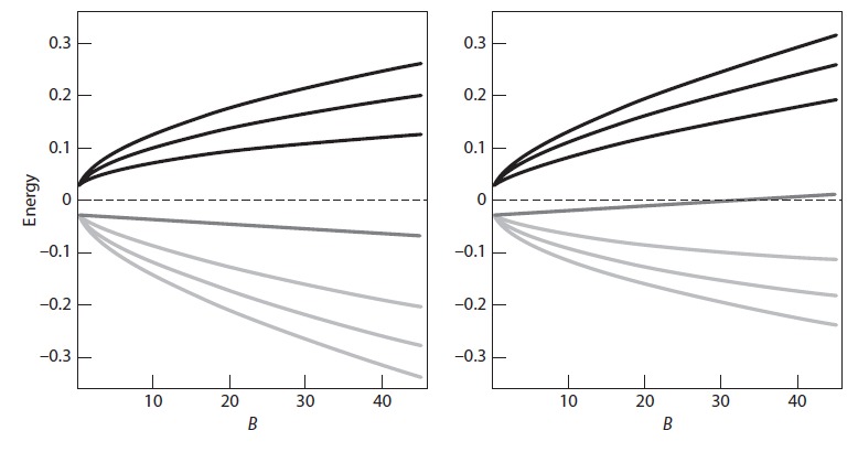
Figure 8.5. Landau-level behavior versus magnetic field \(B\) (only a few Landau levels are plotted) of a Chern Insulator (half of a quantum spin Hall state). Left: Topologically trivial Chern insulator. Right: Topologically nontrivial Chern insulator.
\(8.8\) Edge Modes and the Dirac Equation
The Dirac Hamiltonian also explicitly shows the existence of edge modes at the boundary of two insulators with different Hall conductance. For \(y>0\), we consider our lattice Dirac model with \(M>0\) (say, \(M=0.1\) ), whereas for \(y<0\), we consider our lattice Dirac model with \(-2<\) \(M<0\) (say \(M=-0.1\) ). The only difference between the two lattice Hamiltonians is close to the point \(\Gamma\), where the two continuum Hamiltonians are of Dirac form with negative and positive mass. Hence, in the continuum, the boundary between regions of Hall conductance 0 and Hall conductance 1 is modeled as a boundary between a Dirac fermion with Hall conductance \(-\frac{1}{2}\) and a Dirac fermion with hall conductance \(+\frac{1}{2}\). The moral of the story is that differences in Hall conductance not absolute values are important for edge states.
Let us now formalize the problem. We pick a boundary between a Dirac Hamiltonian with positive mass and one with negative mass in two dimensions-we could have picked any arbitrary dimension because the problem becomes one dimensional after Fourier-transforming in the directions parallel to the translationally invariant interface: \[ H(y)=-i \partial_{x} \sigma_{x}-i \partial_{y} \sigma_{y}+m(y) \sigma_{z} \] where \(m(y)>0\) for \(y>0\) and \(m(y)<0\) for \(y<0 .\) In fact, we need this to be true only at infinity, i.e., \(m(y)>0\) for \(y \rightarrow+\infty\) and \(m(y)<0\) for \(y \rightarrow-\infty\). Different interpolations of \(m(y)\) would physically correspond to different boundary conditions. We look for a wavefunction solution: \[ \psi(x, y)=\phi_{1}(x) \phi_{2}(y), \] which is separable, as the Hamiltonian indicates. We also look for a solution localized on the interface, because our previous experience indicates that boundaries between states of different Hall conductance carry gapless modes. This solution must be dependent on the only length scale in the problem, which is the mass gap: \[ \phi_{2}(y)=e^{-\int_{0}^{y} m\left(y^{\prime}\right) d y^{\prime}} \] This solution has the desirable properties that it is localized on the edge and it is well behaved (finite) when \(y\) goes to \(\pm\) infinity. Also \(\phi_{1}(x)\) is a two-component spinor. We look for a chiral mode of energy \(E=k_{x}\). At \(k_{x}=0\), we will find a zero-energy solution. Plugging in \(\psi(x, y)\) into the Schrodinger equation, we get \[ -i \partial_{x} \sigma_{x} \phi_{1}(x)+m(y)\left(i \sigma_{y} \phi_{1}(x)+\sigma_{z} \phi_{1}(x)\right)=E \phi_{1}(x) \] Obviously, for a zero-energy solution (such as the one at \(k_{x}=0\) ), we must cancel the term that depends on the mass, which is \(y\) -dependent and can be made very large by hand. So, we have \[ i \sigma_{y} \phi_{1}(x)+\sigma_{z} \phi_{1}(x)=0 \longrightarrow \sigma_{x} \phi_{1}(x)=-\phi_{1}(x) \] with the solution \(\phi_{1}(x)=\chi(x) \frac{1}{\sqrt{2}}(1,-1)^{T}\) and \(\chi(x)\) a scalar function of \(x\). This scalar function satisfies the equation \[ i \partial_{x} \chi(x)=E \chi(x) . \] The solution \(\chi(x)=e^{i k_{x} x}\) is a chiral propagating mode in the \(x\) -direction of energy \(E=k_{x}\).
8.9 Haldane's Graphene Model
We finish this chapter by introducing what has historically been the first example of a topological insulator, the Chern insulator on the honeycomb lattice. In the late 1980 s Haldane wanted to mimic the integer quantum Hall effect seen in the Landau-level problem while keeping the (full, not magnetic) translational symmetry of the lattice. This is actually rather hard to do because, as we saw, magnetic fields with nonzero flux per plaquette enlarge the unit cell. The unbroken translational symmetry of the lattice is equivalent to having zero (mod \(2 \pi\) ) flux per plaquette, which leads us to the rather paradoxical situation of trying to obtain Landau levels without a nonzero magnetic field. Haldane realized that time-reversal breaking, rather than overall nonzero flux per unit cell, is the essential ingredient of a nonzero Hall conductance. To keep the translational symmetry of the lattice, we need to break time reversal without a net flux per plaquette. The easiest way to do this is to put the magnetic phases on the next-nearest neighbors because going around a plaquettewill not induce any nearest-neighbor phases. The Haldane model is on the honeycomb lattice, and the Hamiltonian is \[ H=t_{1} \sum_{\langle i, j\rangle} c_{i}^{\dagger} c_{j}+t_{2} \sum_{\langle\langle i, j\rangle\rangle} e^{-i v_{i j} \phi} c_{i}^{\dagger} c_{j}+M \sum_{i} \epsilon_{i} c_{i}^{\dagger} c_{i} \] where \(\epsilon_{i}\) is \(\pm 1\), depending on whether \(i\) is on the \(A\) or \(B\) sublattice, and \(t\) is the nearestneighbor-hopping energy, \(M\) is an on-site inversion symmetry-breaking term, and the new term is the next-nearest neighbor: \[ v_{i j}=\operatorname{sign}\left(\hat{d}_{1} \times \hat{d}_{2}\right)_{z}=\pm 1 \] if \(\hat{d}_{1,2}\) are the vectors along the two bonds constituting the next-nearest neighbors. The signs of the phases \(i \phi\) are shown in figure \(8.6 .\)
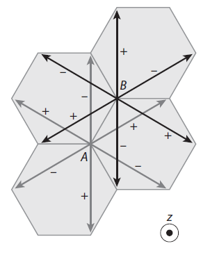
Figure 8.6. Phase convention for the Haldane model for a Chern insulator.
After Fourier transforming, the Haldane Hamiltonian for graphene can be expressed in compact form as \[ h( k )=\epsilon( k )+d_{i}( k ) \sigma_{i} \] where
- \(\epsilon(k)=2 t_{2}\left(\cos (\phi)\left(\cos \left(k \cdot a_{1}\right)+\cos \left(k \cdot a_{1}\right)+\cos \left(k \cdot\left(a_{1}-a_{2}\right)\right)\right)\right.\)
- \(d_{1}( k )=\cos \left( k \cdot a _{1}\right)+\cos \left( k \cdot a _{2}\right)+1\)
- \(d_{2}( k )=\sin \left( k \cdot a _{1}\right)+\sin \left( k \cdot a _{2}\right)\)
- \(d_{3}( k )=M+2 t_{2} \sin (\phi)\left(\sin \left( k \cdot a _{1}\right)-\sin \left( k \cdot a _{2}\right)-\sin \left( k \cdot\left( a _{1}- a _{2}\right)\right)\right) .\)
8.9.1 Symmetry Properties of the Haldane Hamiltonian
We now want to analyze the symmetry properties of the Haldane model. First, we analyze the behavior under time reversal. For time reversal to be satisfied, it would mean that \(\epsilon( k )=\) \(\epsilon(- k ), d_{1}( k )=d_{1}(- k ), d_{2}( k )=-d_{2}(- k )\) and \(d_{3}( k )=d_{3}(- k ) .\) The first three are obviously satisfied by the Haldane Hamiltonian. The last condition is satisfied only for \(\phi=0, \pi\). We now analyze the behavior under inversion. For inversion around the middle of the unit cell (matrix representation \(\sigma_{x}\) ) to be satisfied, it would mean that \(\epsilon( k )=\epsilon(- k ), d_{1}( k )=d_{1}(- k )\), and \(d_{2}( k )=-d_{2}(- k ), d_{3}( k )=-d_{3}(- k )\). The first three are obviously satisfied by the Haldane Hamiltonian, but the last one is satisfied only for \(M=0 .\) For both \(T\) and inversion to be satisfied, we must have both \(\epsilon=0\) and \(\phi=0\) or \(\phi=\pi\).
8.9.2 Phase Diagram of the Haldane Hamiltonian
The interplay between the \(T\) -breaking mass term and the inversion-breaking mass gives the Haldane Hamiltonian, a nontrivial structure with three phases of Hall conductance, \(0,1,-1\), very much like in our square-lattice example. Let us see how. We could directly compute the Hall conductance of the system using our Jacobian formula, but that would not be very physically illuminating. Instead, let us again use the Dirac argument.
We first notice that the system still has \(C_{3}\) symmetry: we have proved before that the Hamiltonian without the new Haldane term has \(C_{3}\) symmetry, and it is trivial to check that the Haldane term is invariant upon the permutation \(\delta _{1} \rightarrow \delta _{2} \rightarrow \delta _{3} \rightarrow \delta _{1}\). The inversion- and \(T\) -breaking terms induce gap in the spectrum, and we can understand the behavior of the model by looking at gap-closing-and-opening transitions. At which point in the \(BZ\) can these transitions happen? Because the model has \(C_{3}\) symmetry, the gap-opening-and-closing transitions (when the system goes gapless) can happen only at the \(K , K ^{\prime}\) points; thus, we focus on the Hamiltonian around those points. We expand the Haldane Hamiltonian around the point \(K\) to linear order: \[ h( K + \kappa )=\epsilon( K )+\kappa_{i} \partial_{i} \in( k = K )+d_{a}( K ) \sigma_{a}+\kappa_{i} \partial_{i} d_{a}( k = K ) \sigma_{a} \] for \(\kappa << K\). After tedious algebraic simplification, we obtain \[ h( K + \kappa )=-3 t_{2} \cos (\phi)+\frac{3}{2} t_{1}\left(\kappa_{y} \sigma_{x}-\kappa_{x} \sigma_{y}\right)+\left(M-3 \sqrt{3} t_{2} \sin (\phi)\right) \sigma_{z} \] Around \(K ^{\prime}\) we have the Hamiltonian \[ h\left( K ^{\prime}+ \kappa \right)=-3 t_{2} \cos (\phi)-\frac{3}{2} t_{1}\left(\kappa_{y} \sigma_{x}+\kappa_{x} \sigma_{y}\right)+\left(M+3 \sqrt{3} t_{2} \sin (\phi)\right) \sigma_{z} \] To obtain the value of the Hall conductance, as we did before, we have to start from a phase where we know the its value and trace the changes in the Chern number as we undergo gapclosing and reopening transitions. Such a phase is easy to find: we start from the case \(M \rightarrow \pm \infty\). In that case the wavefunction is localized on the site \(A\) or \(B\) and the system is trivial, with eigenstates constant in momentum space. As such, the system has no Hall conductance. We pick \(M \rightarrow+\infty\) as a reference point.
The Haldane Hamiltonian is similar to that in equation (8.28) and its Hall conductance can be readily obtained from equation (8.30). Without loss of generality, we now assume \(\phi>0\) (with \(-\pi<\phi<\pi), t_{2}>0\) and start lowering \(M\) from \(+\infty\). At \[ M=3 \sqrt{3} t_{2} \sin \phi \] the \(K\) Dirac fermion goes through a gap-closing-and-opening transition and the Hall conductance changes from (equation \((8.30)) \frac{1}{2} \operatorname{sign}\left(M-3 \sqrt{3} t_{2} \sin (\phi)\right)=\frac{1}{2}\) to \(-\frac{1}{2}\), with a change of Hall conductance equal to \(-1\). The gap at \(K^{\prime}\) stays open for \(M=3 \sqrt{3} t_{2} \sin (\phi)\), and only \(K\) goes through gap-closing-and-reopening transition to give a phase with \[ \sigma_{x y}=-1 \] As we lower \(M\) even more, we reach the value where \[ M=-3 \sqrt{3} t_{2} \sin \phi \] at which point the \(K^{\prime}\) Dirac fermion goes through a gap-closing and re-opening transition, which changes the Hall conductance by \(\Delta \sigma_{x y}=1\) (the point \(K\) remains gapped). The change in Hall conductance means that the phase \(\sigma_{x y}=-1\) before the gap closing goes to a phase with \(\sigma_{x y}=0\) after the gap closing and reopening. This is also necessary because the phase \(M<-3 \sqrt{3} t_{2} \sin \phi\) is adiabatically continuable to the state \(M \rightarrow \infty\), which must have zero Hall conductance. The case \(\phi<0\) is treated in a similar fashion to give the phase diagram in figure \(8.7\).
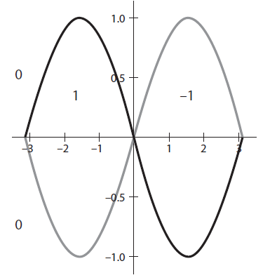
Figure \(8.7\). Phases of the Haldane model. The \(x\) -axis is \(\phi\) and the \(y\) -axis is \(M\). The numbers represent the Hall conductances in the phase. The vertical scale is in units of \(3 \sqrt{3} t_{2}\)